Use temporal functions in formula expressions
Use temporal functions to return values based on timestamps of data points.
Use temporal functions in metrics
In metrics only, you can use the following functions that return values based on timestamps of data points.
Temporal function arguments must be properties from the local asset model or nested expressions. This means that you can't use properties from child asset models in temporal functions.
You can use nested expressions in temporal functions. When you use nested expressions, the following rules apply:
-
Each argument can have only one variable.
For example,
latest( t*9/5 + 32 )is supported. -
Arguments can't be aggregation functions.
For example,
first( sum(x) )isn't supported.
| Function | Description |
|---|---|
|
|
Returns the given variable's value with the earliest timestamp over the current time interval. |
|
|
Returns the given variable's value with the latest timestamp over the current time interval. |
|
|
Returns the given variable's last value before the start of the current time interval. This function computes a data point for every time interval, if the input property has at least one data point in its history. See time-range-defintion for details. |
|
|
Returns the given variable's last value with the latest timestamp before the end of the current time interval. This function computes a data point for every time interval, if the input property has at least one data point in its history. See time-range-defintion for details. |
|
|
Returns the amount of time in seconds that the given variables are positive over the current
time interval. You can use the comparison
functions to create a transform property for the For example, if you have an This function doesn't support metric properties as input variables. This function computes a data point for every time interval, if the input property has at least one data point in its history. |
|
|
Returns the average of input data weighted with time intervals between points. See Time weighted functions parameters for computation and intervals details.The optional argument
|
|
|
Returns the standard deviation of input data weighted with time intervals between points. See Time weighted functions parameters for computation and intervals details. The calculation uses the Last Observed Carry Forward computation algorithm for intervals between data points. In this approach, the data point is computed as the last observed value until the next input data point time stamp. Weight is computed as time interval in seconds between data points or window boundaries. The optional argument
The following formulas are used for computation where:
Equation for population standard deviation: 
Equation for frequency standard deviation: 
|
The following diagram shows how Amazon IoT SiteWise computes the temporal functions
first, last, earliest, and latest, relative to the
current time interval.
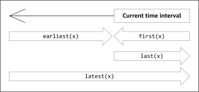
Note
The time range for
first(x),last(x)is (current window start, current window end].The time range for
latest(x)is (beginning of time, current window end].The time range for
earliest(x)is (beginning of time, previous window end].
Time-weighted functions parameters
Time-weighted functions computed for the aggregate window take into account the following:
-
Data points inside the window
-
Time intervals between data points
-
Last data point before the window
-
First data point after the window (for some algorithms)
Terms:
-
Bad data point – Any data point with non-good quality or non-number value. This is not considered in a window result computation.
-
Bad interval – The interval after a bad data point. The interval before the first known data point is also considered a bad interval.
-
Good data point – Any data point with good quality and numeric value.
Note
-
Amazon IoT SiteWise only consumes
GOODquality data when it computes transforms and metrics. It ignoresUNCERTAINandBADdata points. -
The interval before the first known data point is considered a bad interval. See Formula expression tutorials for more information.
The interval after the last known data point continues indefinitely, affecting all following windows. When a new data point arrives, the function recomputes the interval.
Following the rules above, the aggregate window result is computed and limited to window boundaries. By default, the function only sends the window result if the whole window is a good interval.
If the window good interval is smaller than the window length, the function does not send the window.
When the data points affecting the window result change, the function recalculates the window, even if the data points are outside of the window.
If the input property has at least one data point in its history and a computation has been initiated, the function calculates the time-weighted aggregate functions for every time interval.
Example statetime scenario
Consider an example where you have an asset with the following properties:
-
Idle– A measurement that is0or1. When the value is1, the machine is idle. -
Idle Time– A metric that uses the formulastatetime(Idle)to calculate the amount of time in seconds where the machine is idle, per 1 minute interval.
The Idle property has the following data points.
| Timestamp | 2:00:00 PM | 2:00:30 PM | 2:01:15 PM | 2:02:45 PM | 2:04:00 PM |
| Idle | 0 | 1 | 1 | 0 | 0 |
Amazon IoT SiteWise calculates the Idle Time property every minute from the values of
Idle. After this calculation completes, the Idle Time property has the
following data points.
| Timestamp | 2:00:00 PM | 2:01:00 PM | 2:02:00 PM | 2:03:00 PM | 2:04:00 PM |
| Idle Time | N/A | 30 | 60 | 45 | 0 |
Amazon IoT SiteWise performs the following calculations for Idle Time at the end of each
minute.
-
At 2:00 PM (for 1:59 PM to 2:00 PM)
-
There is no data for
Idlebefore 2:00 PM, so no data point is calculated.
-
-
At 2:01 PM (for 2:00 PM to 2:01 PM)
-
At 2:00:00 PM, the machine is active (
Idleis0). -
At 2:00:30 PM, the machine is idle (
Idleis1). -
Idledoesn't change again before the end of the interval at 2:01:00 PM, soIdle Timeis 30 seconds.
-
-
At 2:02 PM (for 2:01 PM to 2:02 PM)
-
At 2:01:00 PM, the machine is idle (per the last data point at 2:00:30 PM).
-
At 2:01:15 PM, the machine is still idle.
-
Idledoesn't change again before the end of the interval at 2:02:00 PM, soIdle Timeis 60 seconds.
-
-
At 2:03 PM (for 2:02 PM to 2:03 PM)
-
At 2:02:00 PM, the machine is idle (per the last data point at 2:01:15 PM).
-
At 2:02:45 PM, the machine is active.
-
Idledoesn't change again before the end of the interval at 2:03:00 PM, soIdle Timeis 45 seconds.
-
-
At 2:04 PM (for 2:03 PM to 2:04 PM)
-
At 2:03:00 PM, the machine is active (per the last data point at 2:02:45 PM).
-
Idledoesn't change again before the end of the interval at 2:04:00 PM, soIdle Timeis 0 seconds.
-
Example TimeWeightedAvg and TimeWeightedStDev scenario
The following tables provide sample inputs and outputs for these one-minute window metrics:
Avg(x), TimeWeightedAvg(x), TimeWeightedAvg(x, "linear"), stDev(x), timeWeightedStDev(x),
                timeWeightedStDev(x, 'p')
.
Sample input for one-minute aggregate window:
Note
These data points all have GOOD quality.
| 03:00:00 | 4.0 |
| 03:01:00 | 2.0 |
| 03:01:10 | 8.0 |
| 03:01:50 | 20.0 |
| 03:02:00 | 14.0 |
| 03:02:05 | 10.0 |
| 03:02:10 | 3.0 |
| 03:02:30 | 20.0 |
| 03:03:30 | 0.0 |
Aggregate results output:
Note
None – Result not produced for this window.
| Time | Avg(x) |
TimeWeightedAvg(x) |
TimeWeightedAvg(X, "linear") |
stDev(X) |
timeWeightedStDev(x) |
timeWeightedStDev(x, 'p') |
|---|---|---|---|---|---|---|
| 3:00:00 | 4 | None | None | 0 | None | None |
| 3:01:00 | 2 | 4 | 3 | 0 | 0 | 0 |
| 3:02:00 | 14 | 9 | 13 | 6 | 5.430610041581775 | 5.385164807134504 |
| 3:03:00 | 11 | 13 | 12.875 | 8.54400374531753 | 7.724054437220943 | 7.659416862050705 |
| 3:04:00 | 0 | 10 | 2.5 | 0 | 10.084389681792215 | 10 |
| 3:05:00 | None | 0 | 0 | None | 0 | 0 |
Use temporal functions in transforms
In transforms only, you can use the
pretrigger() function to retrieve the GOOD quality value
for a variable prior to the property update that initiated the current transform
calculation.
Consider an example where a manufacturer uses Amazon IoT SiteWise to monitor the status of a machine. The manufacturer uses the following measurements and transforms to represent the process:
-
A measurement,
current_state, that can be 0 or 1.-
If the machine is in the cleaning state,
current_stateequals 1. -
If the machine is in the manufacturing state,
current_stateequals 0.
-
-
A transform,
cleaning_state_duration, that equalsif(pretrigger(current_state) == 1, timestamp(current_state) - timestamp(pretrigger(current_state)), none). This transform returns how long the machine has been in the cleaning state in seconds, in the Unix epoch format. For more information, see Use conditional functions in formula expressions and the timestamp() function.
If the machine stays in the cleaning state longer than expected, the manufacturer might investigate the machine.
You can also use the pretrigger() function in multivariate
transforms. For example, you have two measurements named x and
y, and a transform, z, that equals x + y +
pretrigger(y). The following table shows the values for x,
y, and z from 9:00 AM to 9:15 AM.
Note
-
This example assumes that the values for the measurements arrive chronologically. For example, the value of
xfor 09:00 AM arrives before the value ofxfor 09:05 AM. -
If the data points for 9:05 AM arrive before the data points for 9:00 AM,
zisn't calculated at 9:05 AM. -
If the value of
xfor 9:05 AM arrives before the value ofxfor 09:00 AM and the values ofyarrive chronologically,zequals22 = 20 + 1 + 1at 9:05 AM.
| 09:00 AM | 09:05 AM | 09:10 AM | 09:15 AM | |
|---|---|---|---|---|
|
|
10 |
20 |
30 |
|
|
|
1 |
2 |
3 |
|
|
|
|
23 = 20 + 2 + 1
|
25 = 20 + 3 + 2
|
36 = 30 + 3 + 3
|