percentileDiscOver
The percentileDiscOver function calculates the percentile based on the
actual numbers in measure. It uses the grouping and sorting that are
applied in the field wells. The result is partitioned by the specified dimension at the
specified calculation level. The percentileOver function is an alias of
percentileDiscOver.
Use this function to answer the following question: Which actual data points are
present in this percentile? To return the nearest percentile value that is present in
your dataset, use percentileDiscOver. To return an exact percentile value
that might not be present in your dataset, use percentileContOver instead.
Syntax
percentileDiscOver (measure,percentile-n, [partition-by, …] ,calculation-level)
Arguments
- measure
-
Specifies a numeric value to use to compute the percentile. The argument must be a measure or metric. Nulls are ignored in the calculation.
- percentile-n
-
The percentile value can be any numeric constant 0–100. A percentile value of 50 computes the median value of the measure.
- partition-by
-
(Optional) One or more dimensions that you want to partition by, separated by commas. Each field in the list is enclosed in { } (curly braces), if it is more than one word. The entire list is enclosed in [ ] (square brackets).
- calculation-level
-
Specifies where to perform the calculation in relation to the order of evaluation. There are three supported calculation levels:
-
PRE_FILTER
-
PRE_AGG
-
POST_AGG_FILTER (default) – To use this calculation level, you need to specify an aggregation on
measure, for examplesum(measure).
PRE_FILTER and PRE_AGG are applied before the aggregation occurs in a visualization. For these two calculation levels, you can't specify an aggregation on
measurein the calculated field expression. To learn more about calculation levels and when they apply, see Order of evaluation in Amazon Quick and Using level-aware calculations in Quick. -
Returns
The result of the function is a number.
Example of percentileDiscOver
The following example helps explain how percentileDiscOver works.
Example Comparing calculation levels for the median
The following example shows the median for a dimension (category) by using
different calculation levels with the percentileDiscOver function.
The percentile is 50. The dataset is filtered by a region field. The code for
each calculated field is as follows:
-
example = left((A simplified example.)category, 1 ) -
pre_agg = percentileDiscOver ( {Revenue} , 50 , [ example ] , PRE_AGG) -
pre_filter = percentileDiscOver ( {Revenue} , 50 , [ example ] , PRE_FILTER) -
post_agg_filter = percentileDiscOver ( sum ( {Revenue} )
								, 50 , [ example ], POST_AGG_FILTER )
example   pre_filter     pre_agg      post_agg_filter
------------------------------------------------------
0            106,728     119,667            4,117,579
1            102,898      95,946            2,307,547
2             97,629      92,046              554,570
3            100,867     112,585            2,709,057
4             96,416      96,649            3,598,358
5            106,293      97,296            1,875,648
6             97,118      64,395            1,320,672
7             99,915      90,557              969,807
Example The median
The following example calculates the median (the 50th percentile) of
Sales partitioned by City and State.
percentileDiscOver
(
  Sales,
  50,
  [City, State]
)
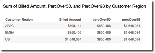
The following example calculates the 98th percentile of sum({Billed
Amount}) partitioned by Customer Region. The fields in
the table calculation are in the field wells of the visual.
percentileDiscOver
(
  sum({Billed Amount}),
  98,
  [{Customer Region}]
)
The following screenshot shows the how these two examples look on a chart.