Analysis Results
Note
After careful consideration, we have made the decision to close new customer access to Amazon Sagemaker Clarify, effective 7/30/26. Existing customers can continue to use the service as normal. Amazon continues to invest in security and availability improvements for Clarify, but we do not plan to introduce new features. For more information, see Clarify availability change.
After a SageMaker Clarify processing job is finished, you can download the output files to inspect them, or you can visualize the results in SageMaker Studio Classic. The following topic describes the analysis results that SageMaker Clarify generates, such as the schema and the report that's generated by bias analysis, SHAP analysis, computer vision explainability analysis, and partial dependence plots (PDPs) analysis. If the configuration analysis contains parameters to compute multiple analyses, then the results are aggregated into one analysis and one report file.
The SageMaker Clarify processing job output directory contains the following files:
-
analysis.json– A file that contains bias metrics and feature importance in JSON format. -
report.ipynb– A static notebook that contains code to help you visualize bias metrics and feature importance. -
explanations_shap/out.csv– A directory that is created and contains automatically generated files based on your specific analysis configurations. For example, if you activate thesave_local_shap_valuesparameter, then per-instance local SHAP values will be saved to theexplanations_shapdirectory. As another example, if youranalysis configurationdoes not contain a value for the SHAP baseline parameter, the SageMaker Clarify explainability job computes a baseline by clustering the input dataset. It then saves the generated baseline to the directory.
For more detailed information, see the following sections.
Topics
Bias analysis
Amazon SageMaker Clarify uses the terminology documented in Amazon SageMaker Clarify Terms for Bias and Fairness to discuss bias and fairness.
Schema for the analysis file
The analysis file is in JSON format and is organized into two sections: pre-training bias metrics and post-training bias metrics. The parameters for pre-training and post-training bias metrics are as follows.
-
pre_training_bias_metrics – Parameters for pre-training bias metrics. For more information, see Pre-training Bias Metrics and Analysis Configuration Files.
-
label – The ground truth label name defined by the
labelparameter of the analysis configuration. -
label_value_or_threshold – A string containing the label values or interval defined by the
label_values_or_thresholdparameter of the analysis configuration. For example, if value1is provided for binary classification problem, then the string will be1. If multiple values[1,2]are provided for multi-class problem, then the string will be1,2. If a threshold40is provided for regression problem, then the string will be an internal like(40, 68]in which68is the maximum value of the label in the input dataset. -
facets – The section contains several key-value pairs, where the key corresponds to the facet name defined by the
name_or_indexparameter of the facet configuration, and the value is an array of facet objects. Each facet object has the following members:-
value_or_threshold – A string containing the facet values or interval defined by the
value_or_thresholdparameter of the facet configuration. -
metrics – The section contains an array of bias metric elements, and each bias metric element has the following attributes:
-
name – The short name of the bias metric. For example,
CI. -
description – The full name of the bias metric. For example,
Class Imbalance (CI). -
value – The bias metric value, or JSON null value if the bias metric is not computed for a particular reason. The values ±∞ are represented as strings
∞and-∞respectively. -
error – An optional error message that explains why the bias metric was not computed.
-
-
-
-
post_training_bias_metrics – The section contains the post-training bias metrics and it follows a similar layout and structure to the pre-training section. For more information, see Post-training Data and Model Bias Metrics.
The following is an example of an analysis configuration that will calculate both pre-training and post-training bias metrics.
{
    "version": "1.0",
    "pre_training_bias_metrics": {
        "label": "Target",
        "label_value_or_threshold": "1",
        "facets": {
            "Gender": [{
                "value_or_threshold": "0",
                "metrics": [
                    {
                        "name": "CDDL",
                        "description": "Conditional Demographic Disparity in Labels (CDDL)",
                        "value": -0.06
                    },
                    {
                        "name": "CI",
                        "description": "Class Imbalance (CI)",
                        "value": 0.6
                    },
                    ...
                ]
            }]
        }
    },
    "post_training_bias_metrics": {
        "label": "Target",
        "label_value_or_threshold": "1",
        "facets": {
            "Gender": [{
                "value_or_threshold": "0",
                "metrics": [
                    {
                        "name": "AD",
                        "description": "Accuracy Difference (AD)",
                        "value": -0.13
                    },
                    {
                        "name": "CDDPL",
                        "description": "Conditional Demographic Disparity in Predicted Labels (CDDPL)",
                        "value": 0.04
                    },
                    ...
                ]
            }]
        }
    }
}
Bias analysis report
The bias analysis report includes several tables and diagrams that contain
detailed explanations and descriptions. These include, but are not limited to, the
distribution of label values, the distribution of facet values, high-level model
performance diagram, a table of bias metrics, and their descriptions. For more
information about bias metrics and how to interpret them, see the Learn How Amazon SageMaker Clarify Helps Detect Bias
SHAP analysis
SageMaker Clarify processing jobs use the Kernel SHAP algorithm to compute feature attributions. The SageMaker Clarify processing job produces both local and global SHAP values. These help to determine the contribution of each feature towards model predictions. Local SHAP values represent the feature importance for each individual instance, while global SHAP values aggregate the local SHAP values across all instances in the dataset. For more information about SHAP values and how to interpret them, see Feature Attributions that Use Shapley Values.
Schema for the SHAP analysis file
Global SHAP analysis results are stored in the explanations section of the
analysis file, under the kernel_shap method. The different parameters
of the SHAP analysis file are as follows:
-
explanations – The section of the analysis file that contains the feature importance analysis results.
-
kernal_shap – The section of the analysis file that contains the global SHAP analysis result.
-
global_shap_values – A section of the analysis file that contains several key-value pairs. Each key in the key-value pair represents a feature name from the input dataset. Each value in the key-value pair corresponds to the feature's global SHAP value. The global SHAP value is obtained by aggregating the per-instance SHAP values of the feature using the
agg_methodconfiguration. If theuse_logitconfiguration is activated, then the value is calculated using the logistic regression coefficients, which can be interpreted as log-odds ratios. -
expected_value – The mean prediction of the baseline dataset. If the
use_logitconfiguration is activated, then the value is calculated using the logistic regression coefficients. -
global_top_shap_text – Used for NLP explainability analysis. A section of the analysis file that includes a set of key-value pairs. SageMaker Clarify processing jobs aggregate the SHAP values of each token and then select the top tokens based on their global SHAP values. The
max_top_tokensconfiguration defines the number of tokens to be selected.Each of the selected top tokens has a key-value pair. The key in the key-value pair corresponds to a top token’s text feature name. Each value in the key-value pair is the global SHAP values of the top token. For an example of a
global_top_shap_textkey-value pair, see the following output.
-
-
The following example shows output from the SHAP analysis of a tabular dataset.
{
    "version": "1.0",
    "explanations": {
        "kernel_shap": {
            "Target": {
                 "global_shap_values": {
                    "Age": 0.022486410860333206,
                    "Gender": 0.007381025261958729,
                    "Income": 0.006843906804137847,
                    "Occupation": 0.006843906804137847,
                    ...
                },
                "expected_value": 0.508233428001
            }
        }
    }
}
The following example shows output from the SHAP analysis of a text dataset. The
output corresponding to the column Comments is an example of output
that is generated after analysis of a text feature.
{
    "version": "1.0",
    "explanations": {
        "kernel_shap": {
            "Target": {
               "global_shap_values": {
                    "Rating": 0.022486410860333206,
                    "Comments": 0.058612104851485144,
                    ...
                },
                "expected_value": 0.46700941970297033,
                "global_top_shap_text": {
                    "charming": 0.04127962903247833,
                    "brilliant": 0.02450240786522321,
                    "enjoyable": 0.024093569652715457,
                    ...
                }
            }
        }
    }
}
Schema for the generated baseline file
When a SHAP baseline configuration is not provided, the SageMaker Clarify processing job
generates a baseline dataset. SageMaker Clarify uses a distance-based clustering algorithm to
generate a baseline dataset from clusters
created
from the input dataset. The resulting baseline dataset is saved
in a CSV file, located at explanations_shap/baseline.csv. This output
file contains a header row and several instances based on the
num_clusters parameter that is specified in the analysis
configuration. The baseline dataset only consists of feature columns. The following
example shows a baseline created by clustering the input dataset.
Age,Gender,Income,Occupation
35,0,2883,1
40,1,6178,2
42,0,4621,0
Schema for local SHAP values from tabular dataset explainability analysis
For tabular datasets, if a single compute instance is used, the SageMaker Clarify processing
job saves the local SHAP values to a CSV file named
explanations_shap/out.csv. If you use multiple compute instances,
local SHAP values are saved to several CSV files in the
explanations_shap directory.
An output file containing local SHAP values has a row containing the local SHAP
values for each column that is defined by the headers. The headers follow the naming
convention of Feature_Label where the feature name is appended by an
underscore, followed by the name of the your target variable.
For multi-class problems, the feature names in the header vary first, then labels.
For example, two features F1, F2, and two classes L1 and
L2, in headers are F1_L1, F2_L1,
F1_L2, and F2_L2. If the analysis configuration
contains a value for the joinsource_name_or_index parameter, then the
key column used in the join is appended to the end of the header name. This allows
mapping of the local SHAP values to instances of the input dataset. An example of an
output file containing SHAP values follows.
Age_Target,Gender_Target,Income_Target,Occupation_Target
0.003937908,0.001388849,0.00242389,0.00274234
-0.0052784,0.017144491,0.004480645,-0.017144491
...
Schema for local SHAP values from NLP explainability analysis
For NLP explainability analysis, if a single compute instance is used, the SageMaker Clarify
processing job saves local SHAP values to a JSON Lines file named
explanations_shap/out.jsonl. If you use multiple compute instances,
the local SHAP values are saved to several JSON Lines files in the
explanations_shap directory.
Each file containing local SHAP values has several data lines, and each line is a valid JSON object. The JSON object has the following attributes:
-
explanations – The section of the analysis file that contains an array of Kernel SHAP explanations for a single instance. Each element in the array has the following members:
-
feature_name – The header name of the features provided by the headers configuration.
-
data_type – The feature type inferred by the SageMaker Clarify processing job. Valid values for text features include
numerical,categorical, andfree_text(for text features). -
attributions – A feature-specific array of attribution objects. A text feature can have multiple attribution objects, each for a unit defined by the
granularityconfiguration. The attribution object has the following members:-
attribution – A class-specific array of probability values.
-
description – (For text features) The description of the text units.
-
partial_text – The portion of the text explained by the SageMaker Clarify processing job.
-
start_idx – A zero-based index to identify the array location indicating the beginning of the partial text fragment.
-
-
-
The following is an example of a single line from a local SHAP values file, beautified to enhance its readability.
{
    "explanations": [
        {
            "feature_name": "Rating",
            "data_type": "categorical",
            "attributions": [
                {
                    "attribution": [0.00342270632248735]
                }
            ]
        },
        {
            "feature_name": "Comments",
            "data_type": "free_text",
            "attributions": [
                {
                    "attribution": [0.005260534499999983],
                    "description": {
                        "partial_text": "It's",
                        "start_idx": 0
                    }
                },
                {
                    "attribution": [0.00424190349999996],
                    "description": {
                        "partial_text": "a",
                        "start_idx": 5
                    }
                },
                {
                    "attribution": [0.010247314500000014],
                    "description": {
                        "partial_text": "good",
                        "start_idx": 6
                    }
                },
                {
                    "attribution": [0.006148907500000005],
                    "description": {
                        "partial_text": "product",
                        "start_idx": 10
                    }
                }
            ]
        }
    ]
}
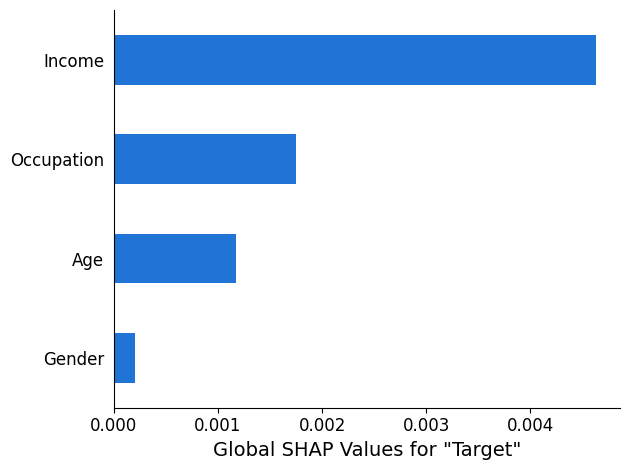
SHAP analysis report
The SHAP analysis report provides a bar chart of a maximum of 10 top
global SHAP values. The following chart example shows the SHAP values for the top
4 features.
Computer vision (CV) explainability analysis
SageMaker Clarify computer vision explainability takes a dataset consisting of images and treats each image as a collection of super pixels. After analysis, the SageMaker Clarify processing job outputs a dataset of images where each image shows the heat map of the super pixels.
The following example shows an input speed limit sign on the left and a heat map shows
the magnitude of SHAP values on the right. These SHAP values were calculated by an image
recognition Resnet-18 model that is trained to recognize German traffic signs
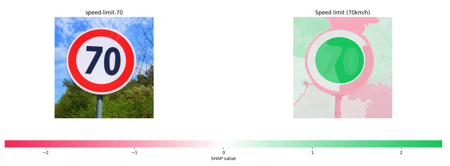
For more information, see the sample notebooks Explaining Image Classification with SageMaker Clarify
Partial dependence plots (PDPs) analysis
Partial dependence plots show the dependence of the predicted target response on a set of input features of interest. These are marginalized over the values of all other input features and are referred to as the complement features. Intuitively, you can interpret the partial dependence as the target response, which is expected as a function of each input feature of interest.
Schema for the analysis file
The PDP values are stored in the explanations section of the analysis
file under the pdp method. The parameters for explanations
are as follows:
-
explanations – The section of the analysis files that contains feature importance analysis results.
-
pdp – The section of the analysis file that contains an array of PDP explanations for a single instance. Each element of the array has the following members:
-
feature_name – The header name of the features provided by the
headersconfiguration. -
data_type – The feature type inferred by the SageMaker Clarify processing job. Valid values for
data_typeinclude numerical and categorical. -
feature_values – Contains the values present in the feature. If the
data_typeinferred by SageMaker Clarify is categorical,feature_valuescontains all of the unique values that the feature could be. If thedata_typeinferred by SageMaker Clarify is numerical,feature_valuescontains a list of the central value of generated buckets. Thegrid_resolutionparameter determines the number of buckets used to group the feature column values. -
data_distribution – An array of percentages, where each value is the percentage of instances that a bucket contains. The
grid_resolutionparameter determines the number of buckets. The feature column values are grouped into these buckets. -
model_predictions – An array of model predictions, where each element of the array is an array of predictions that corresponds to one class in the model’s output.
label_headers – The label headers provided by the
label_headersconfiguration. -
error – An error message generated if the PDP values are not computed for a particular reason. This error message replaces the content contained in the
feature_values,data_distributions, andmodel_predictionsfields.
-
-
The following is example output from an analysis file containing a PDP analysis result.
{
    "version": "1.0",
    "explanations": {
        "pdp": [
            {
                "feature_name": "Income",
                "data_type": "numerical",
                "feature_values": [1046.9, 2454.7, 3862.5, 5270.2, 6678.0, 8085.9, 9493.6, 10901.5, 12309.3, 13717.1],
                "data_distribution": [0.32, 0.27, 0.17, 0.1, 0.045, 0.05, 0.01, 0.015, 0.01, 0.01],
                "model_predictions": [[0.69, 0.82, 0.82, 0.77, 0.77, 0.46, 0.46, 0.45, 0.41, 0.41]],
                "label_headers": ["Target"]
            },
            ...
        ]
    }
}
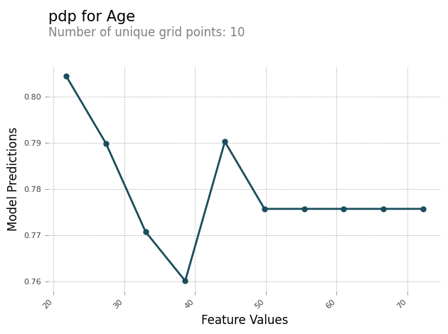
PDP analysis report
You can generate an analysis report containing a PDP chart for each feature. The
PDP chart plots feature_values along the x-axis, and it plots
model_predictions along the y-axis. For multi-class models,
model_predictions is an array, and each element of this array
corresponds to one of the model prediction classes.
The following is an example of PDP chart for the feature Age. In the
example output, the PDP shows the number of feature values that are grouped into
buckets. The number of buckets is determined by grid_resolution. The
buckets of feature values are plotted against model predictions. In this example,
the higher feature values have the same model prediction values.