Get Insights On Data and Data Quality - Amazon SageMaker
Services or capabilities described in Amazon Web Services documentation might vary by Region. To see the differences applicable to the China Regions, see Getting Started with Amazon Web Services in China (PDF).

Get Insights On Data and Data Quality

Use the Data Quality and Insights Report to perform an analysis of the data that you've imported into Data Wrangler. We recommend that you create the report after you import your dataset. You can use the report to help you clean and process your data. It gives you information such as the number of missing values and the number of outliers. If you have issues with your data, such as target leakage or imbalance, the insights report can bring those issues to your attention.

Use the following procedure to create a Data Quality and Insights report. It assumes that you've already imported a dataset into your Data Wrangler flow.

To create a Data Quality and Insights report
  1. Choose a + next to a node in your Data Wrangler flow.

  2. Select Get data insights.

  3. For Analysis name, specify a name for the insights report.

  4. (Optional) For Target column, specify the target column.

  5. For Problem type, specify Regression or Classification.

  6. For Data size, specify one of the following:

    • 50 K – Uses the first 50000 rows of the dataset that you've imported to create the report.

    • Entire dataset – Uses the entire dataset that you've imported to create the report.

    Note

    Creating a Data Quality and Insights report on the entire dataset uses an Amazon SageMaker processing job. A SageMaker processing job provisions the additional compute resources required to get insights for all of your data. For more information about SageMaker processing jobs, see Process data.

  7. Choose Create.

The following topics show the sections of the report:

You can either download the report or view it online. To download the report, choose the download button at the top right corner of the screen. The following image shows the button.

Summary

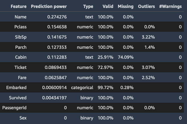
The insights report has a brief summary of the data that includes general information such as missing values, invalid values, feature types, outlier counts, and more. It can also include high severity warnings that point to probable issues with the data. We recommend that you investigate the warnings.

The following is an example of a report summary.

Target column

When you create the data quality and insights report, Data Wrangler gives you the option to select a target column. A target column is a column that you're trying to predict. When you choose a target column, Data Wrangler automatically creates a target column analysis. It also ranks the features in the order of their predictive power. When you select a target column, you must specify whether you’re trying to solve a regression or a classification problem.

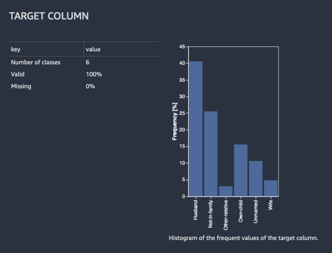
For classification, Data Wrangler shows a table and a histogram of the most common classes. A class is a category. It also presents observations, or rows, with a missing or invalid target value.

The following image shows an example target column analysis for a classification problem.

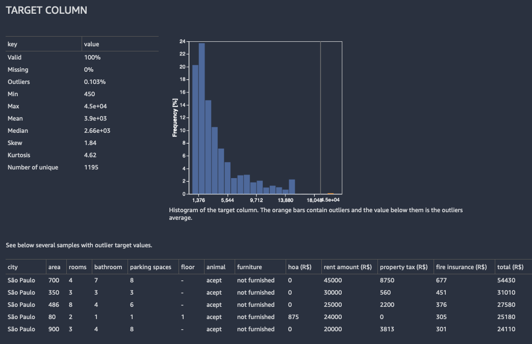
For regression, Data Wrangler shows a histogram of all the values in the target column. It also presents observations, or rows, with a missing, invalid, or outlier target value.

The following image shows an example target column analysis for a regression problem.
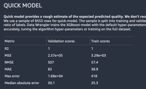
Quick model

The Quick model provides an estimate of the expected predicted quality of a model that you train on your data.

Data Wrangler splits your data into training and validation folds. It uses 80% of the samples for training and 20% of the values for validation. For classification, the sample is stratified split. For a stratified split, each data partition has the same ratio of labels. For classification problems, it's important to have the same ratio of labels between the training and classification folds. Data Wrangler trains the XGBoost model with the default hyperparameters. It applies early stopping on the validation data and performs minimal feature preprocessing.

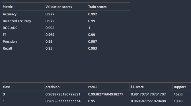
For classification models, Data Wrangler returns both a model summary and a confusion matrix.

The following is an example of a classification model summary. To learn more about the information that it returns, see Definitions.

The following is an example of a confusion matrix that the quick model returns.

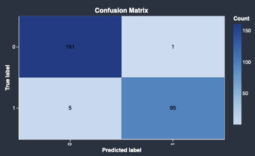
A confusion matrix gives you the following information:

  • The number of times the predicted label matches the true label.

  • The number of times the predicted label doesn't match the true label.

The true label represents an actual observation in your data. For example, if you're using a model to detect fraudulent transactions, the true label represents a transaction that is actually fraudulent or non-fraudulent. The predicted label represents the label that your model assigns to the data.

You can use the confusion matrix to see how well the model predicts the presence or the absence of a condition. If you're predicting fraudulent transactions, you can use the confusion matrix to get a sense of both the sensitivity and the specificity of the model. The sensitivity refers to the model's ability to detect fraudulent transactions. The specificity refers to the model's ability to avoid detecting non-fraudulent transactions as fraudulent.

The following is an example of the quick model outputs for a regression problem.
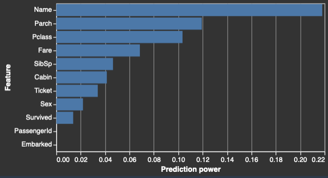
Feature summary

When you specify a target column, Data Wrangler orders the features by their prediction power. Prediction power is measured on the data after it was split into 80% training and 20% validation folds. Data Wrangler fits a model for each feature separately on the training fold. It applies minimal feature preprocessing and measures prediction performance on the validation data.

It normalizes the scores to the range [0,1]. Higher prediction scores indicate columns that are more useful for predicting the target on their own. Lower scores point to columns that aren’t predictive of the target column.

It’s uncommon for a column that isn’t predictive on its own to be predictive when it’s used in tandem with other columns. You can confidently use the prediction scores to determine whether a feature in your dataset is predictive.

A low score usually indicates the feature is redundant. A score of 1 implies perfect predictive abilities, which often indicates target leakage. Target leakage usually happens when the dataset contains a column that isn’t available at the prediction time. For example, it could be a duplicate of the target column.

The following are examples of the table and the histogram that show the prediction value of each feature.

Samples

Data Wrangler provides information about whether your samples are anomalous or if there are duplicates in your dataset.

Data Wrangler detects anomalous samples using the isolation forest algorithm. The isolation forest associates an anomaly score with each sample (row) of the dataset. Low anomaly scores indicate anomalous samples. High scores are associated with non-anomalous samples. Samples with a negative anomaly score are usually considered anomalous and samples with positive anomaly score are considered non-anomalous.

When you look at a sample that might be anomalous, we recommend that you pay attention to unusual values. For example, you might have anomalous values that result from errors in gathering and processing the data. The following is an example of the most anomalous samples according to the Data Wrangler’s implementation of the isolation forest algorithm. We recommend using domain knowledge and business logic when you examine the anomalous samples.

Data Wrangler detects duplicate rows and calculates the ratio of duplicate rows in your data. Some data sources could include valid duplicates. Other data sources could have duplicates that point to problems in data collection. Duplicate samples that result from faulty data collection could interfere with machine learning processes that rely on splitting the data into independent training and validation folds.

The following are elements of the insights report that can be impacted by duplicated samples:

  • Quick model

  • Prediction power estimation

  • Automatic hyperparameter tuning

You can remove duplicate samples from the dataset using the Drop duplicates transform under Manage rows. Data Wrangler shows you the most frequently duplicated rows.

Definitions

The following are definitions for the technical terms that are used in the data insights report.

Feature types

The following are the definitions for each of the feature types:

  • Numeric – Numeric values can be either floats or integers, such as age or income. The machine learning models assume that numeric values are ordered and a distance is defined over them. For example, 3 is closer to 4 than to 10 and 3 < 4 < 10.

  • Categorical – The column entries belong to a set of unique values, which is usually much smaller than the number of entries in the column. For example, a column of length 100 could contain the unique values Dog, Cat, and Mouse. The values could be numeric, text, or a combination of both. Horse, House, 8, Love, and 3.1 would all be valid values and could be found in the same categorical column. The machine learning model does not assume order or distance on the values of categorical features, as opposed to numeric features, even when all the values are numbers.

  • Binary – Binary features are a special categorical feature type in which the cardinality of the set of unique values is 2.

  • Text – A text column contains many non-numeric unique values. In extreme cases, all the elements of the column are unique. In an extreme case, no two entries are the same.

  • Datetime – A datetime column contains information about the date or time. It can have information about both the date and time.

Feature statistics

The following are definitions for each of the feature statistics:

  • Prediction power – Prediction power measures how useful the column is in predicting the target.

  • Outliers (in numeric columns) – Data Wrangler detects outliers using two statistics that are robust to outliers: median and robust standard deviation (RSTD). RSTD is derived by clipping the feature values to the range [5 percentile, 95 percentile] and calculating the standard deviation of the clipped vector. All values larger than median + 5 * RSTD or smaller than median - 5 * RSTD are considered to be outliers.

  • Skew (in numeric columns) – Skew measures the symmetry of the distribution and is defined as the third moment of the distribution divided by the third power of the standard deviation. The skewness of the normal distribution or any other symmetric distribution is zero. Positive values imply that the right tail of the distribution is longer than the left tail. Negative values imply that the left tail of the distribution is longer than the right tail. As a rule of thumb, a distribution is considered skewed when the absolute value of the skew is larger than 3.

  • Kurtosis (in numeric columns) – Pearson's kurtosis measures the heaviness of the tail of the distribution. It's defined as the fourth moment of the distribution divided by the square of the second moment. The kurtosis of the normal distribution is 3. Kurtosis values lower than 3 imply that the distribution is concentrated around the mean and the tails are lighter than the tails of the normal distribution. Kurtosis values higher than 3 imply heavier tails or outliers.

  • Missing values – Null-like objects, empty strings and strings composed of only white spaces are considered missing.

  • Valid values for numeric features or regression target – All values that you can cast to finite floats are valid. Missing values are not valid.

  • Valid values for categorical, binary, or text features, or for classification target – All values that are not missing are valid.

  • Datetime features – All values that you can cast to a datetime object are valid. Missing values are not valid.

  • Invalid values – Values that are either missing or you can't properly cast. For example, in a numeric column, you can't cast the string "six" or a null value.

Quick model metrics for regression

The following are the definitions for the quick model metrics:

  • R2 or coefficient of determination) – R2 is the proportion of the variation in the target that is predicted by the model. R2 is in the range of [-infty, 1]. 1 is the score of the model that predicts the target perfectly and 0 is the score of the trivial model that always predicts the target mean.

  • MSE or mean squared error – MSE is in the range [0, infty]. 0 is the score of the model that predicts the target perfectly.

  • MAE or mean absolute error – MAE is in the range [0, infty] where 0 is the score of the model that predicts the target perfectly.

  • RMSE or root mean square error – RMSE is in the range [0, infty] where 0 is the score of the model that predicts the target perfectly.

  • Max error – The maximum absolute value of the error over the dataset. Max error is in the range [0, infty]. 0 is the score of the model that predicts the target perfectly.

  • Median absolute error – Median absolute error is in the range [0, infty]. 0 is the score of the model that predicts the target perfectly.

Quick model metrics for classification

The following are the definitions for the quick model metrics:

  • Accuracy – Accuracy is the ratio of samples that are predicted accurately. Accuracy is in the range [0, 1]. 0 is the score of the model that predicts all samples incorrectly and 1 is the score of the perfect model.

  • Balanced accuracy – Balanced accuracy is the ratio of samples that are predicted accurately when the class weights are adjusted to balance the data. All classes are given the same importance, regardless of their frequency. Balanced accuracy is in the range [0, 1]. 0 is the score of the model that predicts all samples wrong. 1 is the score of the perfect model.

  • AUC (binary classification) – This is the area under the receiver operating characteristic curve. AUC is in the range [0, 1] where a random model returns a score of 0.5 and the perfect model returns a score of 1.

  • AUC (OVR) – For multiclass classification, this is the area under the receiver operating characteristic curve calculated separately for each label using one versus rest. Data Wrangler reports the average of the areas. AUC is in the range [0, 1] where a random model returns a score of 0.5 and the perfect model returns a score of 1.

  • Precision – Precision is defined for a specific class. Precision is the fraction of true positives out of all the instances that the model classified as that class. Precision is in the range [0, 1]. 1 is the score of the model that has no false positives for the class. For binary classification, Data Wrangler reports the precision of the positive class.

  • Recall – Recall is defined for a specific class. Recall is the fraction of the relevant class instances that are successfully retrieved. Recall is in the range [0, 1]. 1 is the score of the model that classifies all the instances of the class correctly. For binary classification, Data Wrangler reports the recall of the positive class.

  • F1 – F1 is defined for a specific class. It's the harmonic mean of the precision and recall. F1 is in the range [0, 1]. 1 is the score of the perfect model. For binary classification, Data Wrangler reports the F1 for classes with positive values.

Textual patterns

Patterns describe the textual format of a string using an easy to read format. The following are examples of textual patterns:

  • "{digits:4-7}" describes a sequence of digits that have a length between 4 and 7.

  • "{alnum:5}" describes an alpha-numeric string with a length of exactly 5.

Data Wrangler infers the patterns by looking at samples of non-empty strings from your data. It can describe many of the commonly used patterns. The confidence expressed as a percentage indicates how much of the data is estimated to match the pattern. Using the textual pattern, you can see which rows in your data you need to correct or drop.

The following describes the patterns that Data Wrangler can recognize:

Pattern Textual Format

{alnum}

Alphanumeric strings

{any}

Any string of word characters

{digits}

A sequence of digits

{lower}

A lowercase word

{mixed}

A mixed-case word

{name}

A word beginning with a capital letter

{upper}

An uppercase word

{whitespace}

whitespace characters

A word character is either an underscore or a character that might appear in a word in any language. For example, the strings 'Hello_word' and 'écoute' both consist of word characters. 'H' and 'é' are both examples of word characters.