Debugger advanced demos and visualization
The following demos walk you through advanced use cases and visualization scripts using Debugger.
Topics
Training and pruning models with Amazon SageMaker Experiments and Debugger
Using SageMaker Debugger to monitor a convolutional autoencoder model training
Using SageMaker Debugger to monitor attentions in BERT model training
Using SageMaker Debugger to visualize class activation maps in convolutional neural networks (CNNs)
Training and pruning models with Amazon SageMaker Experiments and Debugger
Dr. Nathalie Rauschmayr, Amazon Applied Scientist | Length: 49 minutes 26 seconds
Find out how Amazon SageMaker Experiments and Debugger can simplify the management of your training jobs. Amazon SageMaker Debugger provides transparent visibility into training jobs and saves training metrics into your Amazon S3 bucket. SageMaker Experiments enables you to call the training information as trials through SageMaker Studio and supports visualization of the training job. This helps you keep model quality high while reducing less important parameters based on importance rank.
This video demonstrates a model pruning technique that makes pre-trained ResNet50 and AlexNet models lighter and affordable while keeping high standards for model accuracy.
SageMaker AI Estimator trains those algorithms supplied from the PyTorch model zoo in an Amazon Deep Learning Containers with PyTorch framework, and Debugger extracts training metrics from the training process.
The video also demonstrates how to set up a Debugger custom rule to watch the accuracy of a pruned model, to trigger an Amazon CloudWatch event and an Amazon Lambda function when the accuracy hits a threshold, and to automatically stop the pruning process to avoid redundant iterations.
Learning objectives are as follows:
-
Learn how to use SageMaker AI to accelerate ML model training and improve model quality.
-
Understand how to manage training iterations with SageMaker Experiments by automatically capturing input parameters, configurations, and results.
-
Discover how Debugger makes the training process transparent by automatically capturing real-time tensor data from metrics such as weights, gradients, and activation outputs of convolutional neural networks.
-
Use CloudWatch to trigger Lambda when Debugger catches issues.
-
Master the SageMaker training process using SageMaker Experiments and Debugger.
You can find the notebooks and training scripts used in this video from SageMaker Debugger PyTorch Iterative Model Pruning
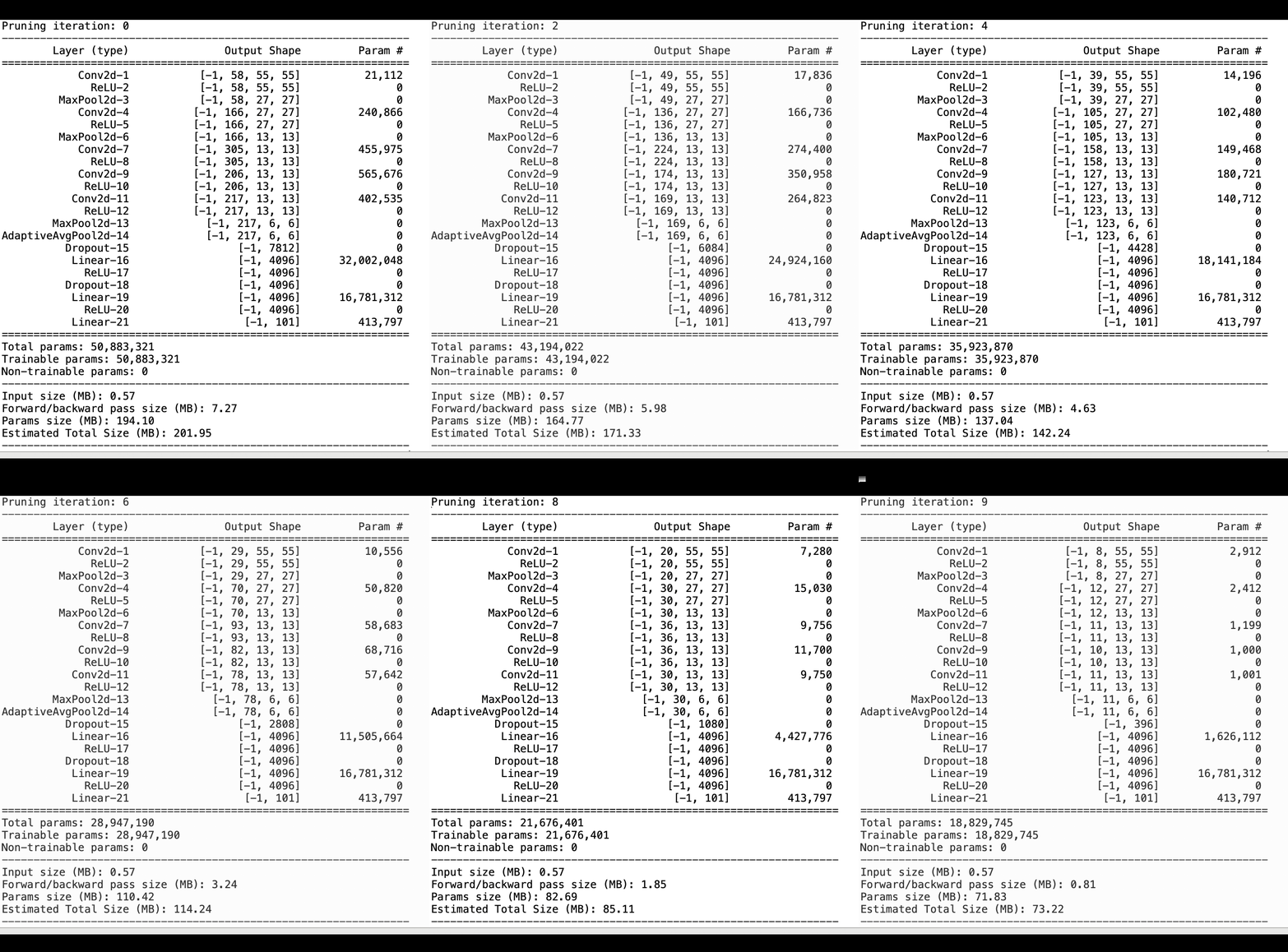
The following image shows how the iterative model pruning process reduces the size of AlexNet by cutting out the 100 least significant filters based on importance rank evaluated by activation outputs and gradients.
The pruning process reduced the initial 50 million parameters to 18 million. It also reduced the estimated model size from 201 MB to 73 MB.
You also need to track model accuracy, and the following image shows how you can plot the model pruning process to visualize changes in model accuracy based on the number of parameters in SageMaker Studio.
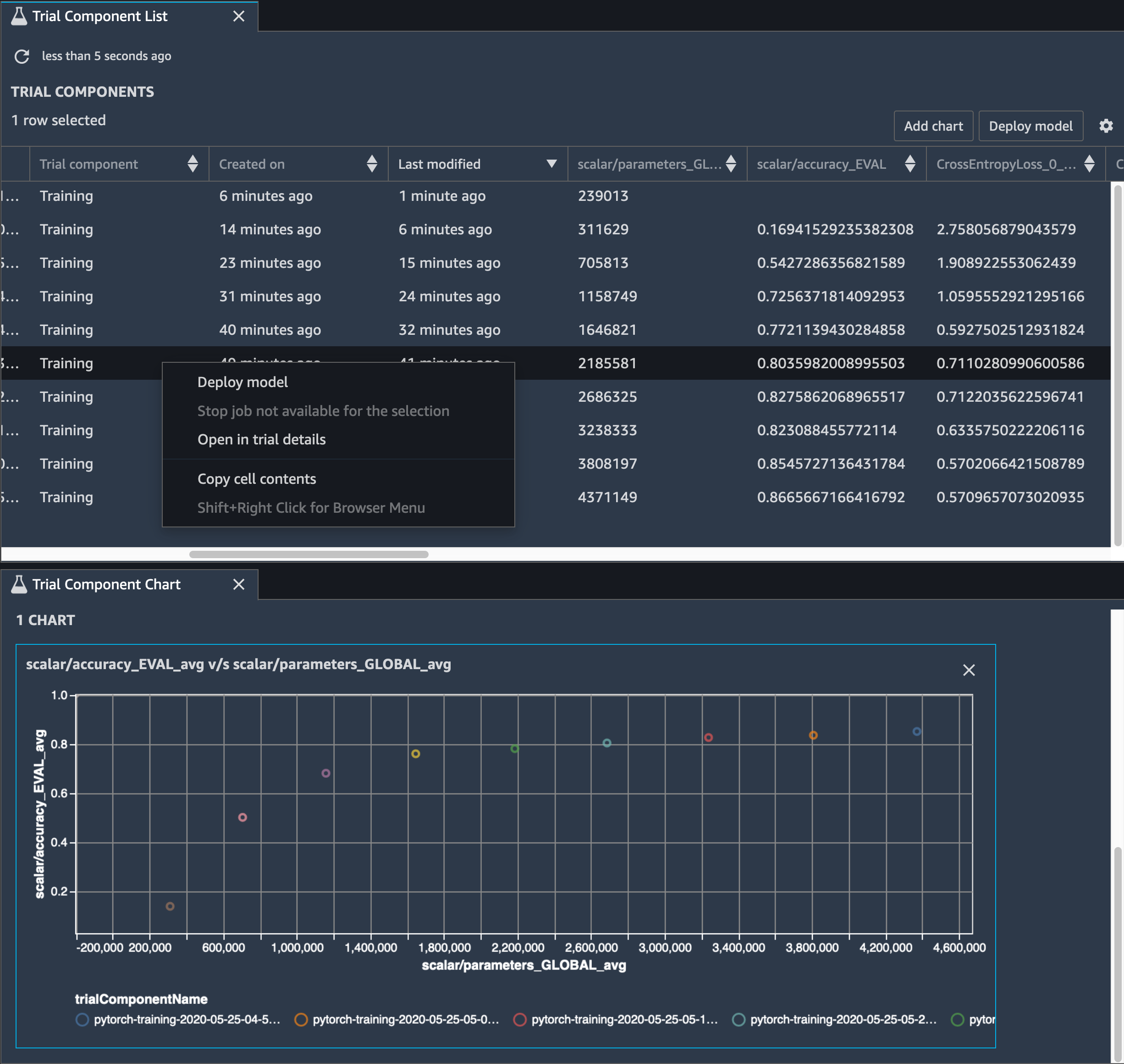
In SageMaker Studio, choose the Experiments tab, select a list of tensors saved by Debugger from the pruning process, and then compose a Trial Component List panel. Select all ten iterations and then choose Add chart to create a Trial Component Chart. After you decide on a model to deploy, choose the trial component and choose a menu to perform an action or choose Deploy model.
Note
To deploy a model through SageMaker Studio using the following notebook example, add a
line at the end of the train function in the
train.py script.
# In the train.py script, look for the train function in line 58. def train(epochs, batch_size, learning_rate): ... print('acc:{:.4f}'.format(correct/total)) hook.save_scalar("accuracy", correct/total, sm_metric=True) # Add the following code to line 128 of the train.py script to save the pruned models # under the current SageMaker Studio model directorytorch.save(model.state_dict(), os.environ['SM_MODEL_DIR'] + '/model.pt')
Using SageMaker Debugger to monitor a convolutional autoencoder model training
This notebook demonstrates how SageMaker Debugger visualizes tensors from an unsupervised (or self-supervised) learning process on a MNIST image dataset of handwritten numbers.
The training model in this notebook is a convolutional autoencoder with the MXNet framework. The convolutional autoencoder has a bottleneck-shaped convolutional neural network that consists of an encoder part and a decoder part.
The encoder in this example has two convolution layers to produce compressed representation (latent variables) of the input images. In this case, the encoder produces a latent variable of size (1, 20) from an original input image of size (28, 28) and significantly reduces the size of data for training by 40 times.
The decoder has two deconvolutional layers and ensures that the latent variables preserve key information by reconstructing output images.
The convolutional encoder powers clustering algorithms with smaller input data size and the performance of clustering algorithms such as k-means, k-NN, and t-Distributed Stochastic Neighbor Embedding (t-SNE).
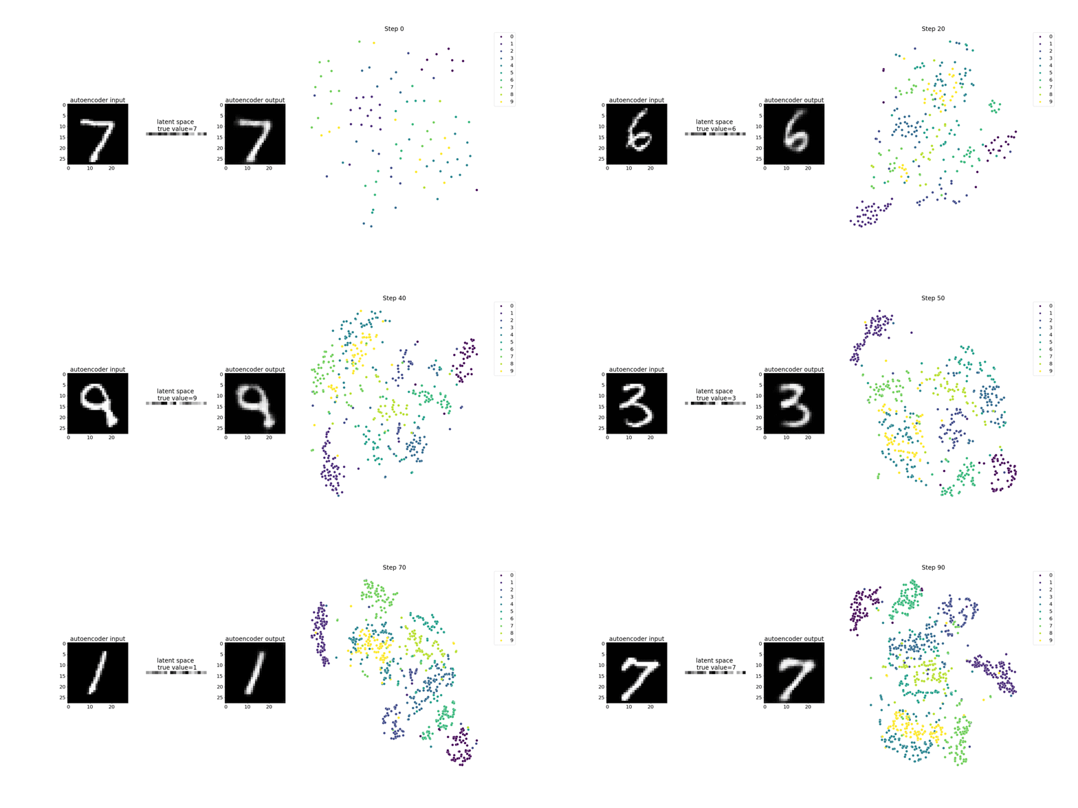
This notebook example demonstrates how to visualize the latent variables using Debugger, as shown in the following animation. It also demonstrates how the t-SNE algorithm classifies the latent variables into ten clusters and projects them into a two-dimensional space. The scatter plot color scheme on the right side of the image reflects the true values to show how well the BERT model and t-SNE algorithm organize the latent variables into the clusters.
Using SageMaker Debugger to monitor attentions in BERT model training
Bidirectional Encode Representations from Transformers (BERT) is a language representation model. As the name of model reflects, the BERT model builds on transfer learning and the Transformer model for natural language processing (NLP).
The BERT model is pre-trained on unsupervised tasks such as predicting missing words in a sentence or predicting the next sentence that naturally follows a previous sentence. The training data contains 3.3 billion words (tokens) of English text, from sources such as Wikipedia and electronic books. For a simple example, the BERT model can give a high attention to appropriate verb tokens or pronoun tokens from a subject token.
The pre-trained BERT model can be fine-tuned with an additional output layer to achieve state-of-the-art model training in NLP tasks, such as automated responses to questions, text classification, and many others.
Debugger collects tensors from the fine-tuning process. In the context of NLP, the weight of neurons is called attention.
This notebook demonstrates how to use the pre-trained BERT model
from the GluonNLP model zoo
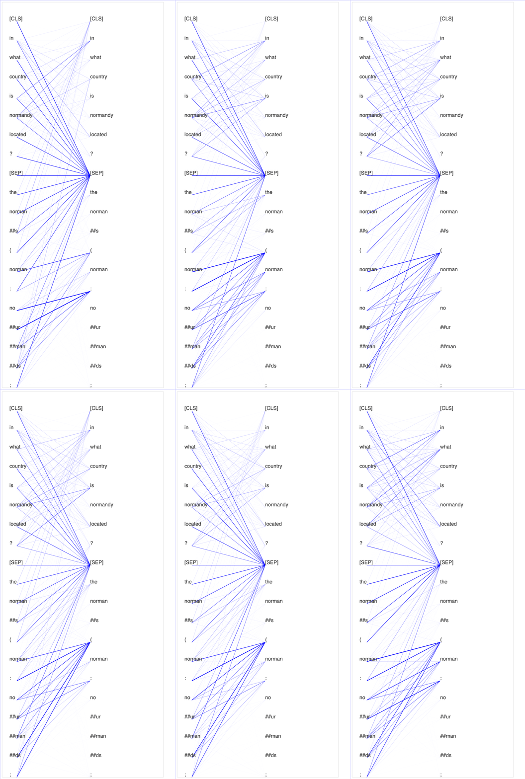
Plotting attention scores and individual neurons in the query and key vectors can help to identify causes of incorrect model predictions. With SageMaker AI Debugger, you can retrieve the tensors and plot the attention-head view in real time as training progresses and understand what the model is learning.
The following animation shows the attention scores of the first 20 input tokens for ten iterations in the training job provided in the notebook example.
Using SageMaker Debugger to visualize class activation maps in convolutional neural networks (CNNs)
This notebook demonstrates how to use SageMaker Debugger to plot class activation maps for image detection and classification in convolutional neural networks (CNNs). In deep learning, a convolutional neural network (CNN or ConvNet) is a class of deep neural networks, most commonly applied to analyzing visual imagery. One of the applications that adopts the class activation maps is self-driving cars, which require instantaneous detection and classification of images such as traffic signs, roads, and obstacles.
In this notebook, the PyTorch ResNet model is trained on the German Traffic Sign Dataset
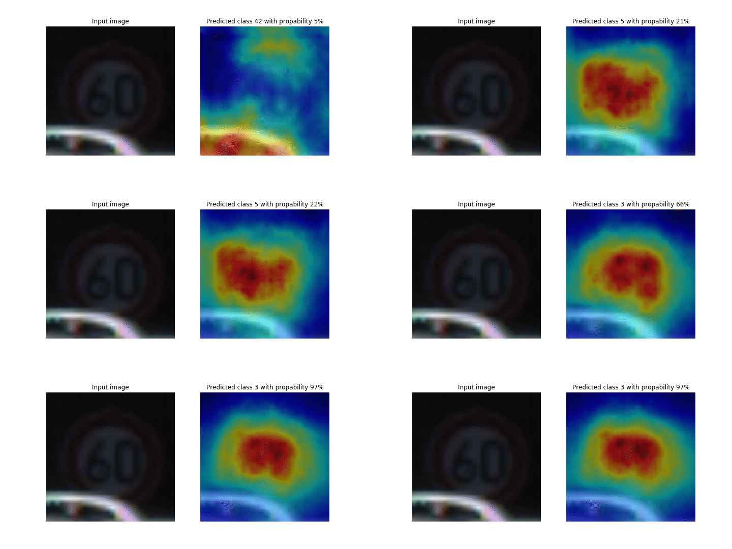
During the training process, SageMaker Debugger collects tensors to plot the class activation maps in real time. As shown in the animated image, the class activation map (also called as a saliency map) highlights regions with high activation in red color.
Using tensors captured by Debugger, you can visualize how the activation map evolves during the model training. The model starts by detecting the edge on the lower-left corner at the beginning of the training job. As the training progresses, the focus shifts to the center and detects the speed limit sign, and the model successfully predicts the input image as Class 3, which is a class of speed limit 60km/h signs, with a 97% confidence level.