Services or capabilities described in Amazon Web Services documentation might vary by Region. To see the differences applicable to the China Regions, see Getting Started with Amazon Web Services in China (PDF).

Access the Sentinel-2 raster data collection and create an earth observation job to perform land segmentation

This Python-based tutorial uses the SDK for Python (Boto3) and an Amazon SageMaker Studio Classic notebook. To complete this demo successfully, make sure that you have the required Amazon Identity and Access Management (IAM) permissions to use SageMaker geospatial and Studio Classic. SageMaker geospatial requires that you have a user, group, or role which can access Studio Classic. You must also have a SageMaker execution role that specifies the SageMaker geospatial service principal, sagemaker-geospatial.amazonaws.com in its trust policy.

To learn more about these requirements, see SageMaker geospatial IAM roles.

This tutorial shows you how to use SageMaker geospatial API to complete the following tasks:

Using list_raster_data_collections to find available data collections

SageMaker geospatial supports multiple raster data collections. To learn more about the available data collections, see Data collections.

This demo uses satellite data that's collected from Sentinel-2 Cloud-Optimized GeoTIFF satellites. These satellites provide global coverage of Earth's land surface every five days. In addition to collecting surface images of Earth, the Sentinel-2 satellites also collect data across a variety of spectralbands.

To search an area of interest (AOI), you need the ARN that's associated with the Sentinel-2 satellite data. To find the available data collections and their associated ARNs in your Amazon Web Services Region, use the list_raster_data_collections API operation.

Because the response can be paginated, you must use the get_paginator operation to return all of the relevant data:

import boto3
import sagemaker
import sagemaker_geospatial_map
import json 

## SageMaker Geospatial  is currently only avaialable in US-WEST-2  
session = boto3.Session(region_name='us-west-2')
execution_role = sagemaker.get_execution_role()

## Creates a SageMaker Geospatial client instance 
geospatial_client = session.client(service_name="sagemaker-geospatial")

# Creates a resusable Paginator for the list_raster_data_collections API operation 
paginator = geospatial_client.get_paginator("list_raster_data_collections")

# Create a PageIterator from the paginator class
page_iterator = paginator.paginate()

# Use the iterator to iterate throught the results of list_raster_data_collections
results = []
for page in page_iterator:
    results.append(page['RasterDataCollectionSummaries'])

print(results)

This is a sample JSON response from the list_raster_data_collections API operation. It's truncated to include only the data collection (Sentinel-2) that's used in this code example. For more details about a specific raster data collection, use get_raster_data_collection:

{
    "Arn": "arn:aws:sagemaker-geospatial:us-west-2:378778860802:raster-data-collection/public/nmqj48dcu3g7ayw8",
    "Description": "Sentinel-2a and Sentinel-2b imagery, processed to Level 2A (Surface Reflectance) and converted to Cloud-Optimized GeoTIFFs",
    "DescriptionPageUrl": "https://registry.opendata.aws/sentinel-2-l2a-cogs",
    "Name": "Sentinel 2 L2A COGs",
    "SupportedFilters": [
        {
            "Maximum": 100,
            "Minimum": 0,
            "Name": "EoCloudCover",
            "Type": "number"
        },
        {
            "Maximum": 90,
            "Minimum": 0,
            "Name": "ViewOffNadir",
            "Type": "number"
        },
        {
            "Name": "Platform",
            "Type": "string"
        }
    ],
    "Tags": {},
    "Type": "PUBLIC"
}

After running the previous code sample, you get the ARN of the Sentinel-2 raster data collection, arn:aws:sagemaker-geospatial:us-west-2:378778860802:raster-data-collection/public/nmqj48dcu3g7ayw8. In the next section, you can query the Sentinel-2 data collection using the search_raster_data_collection API.

Searching the Sentinel-2 raster data collection using search_raster_data_collection

In the preceding section, you used list_raster_data_collections to get the ARN for the Sentinel-2 data collection. Now you can use that ARN to search the data collection over a given area of interest (AOI), time range, properties, and the available UV bands.

To call the search_raster_data_collection API you must pass in a Python dictionary to the RasterDataCollectionQuery parameter. This example uses AreaOfInterest, TimeRangeFilter, PropertyFilters, and BandFilter. For ease, you can specify the Python dictionary using the variable search_rdc_query to hold the search query parameters:

search_rdc_query = {
    "AreaOfInterest": {
        "AreaOfInterestGeometry": {
            "PolygonGeometry": {
                "Coordinates": [
                    [
                        # coordinates are input as longitute followed by latitude 
                        [-114.529, 36.142],
                        [-114.373, 36.142],
                        [-114.373, 36.411],
                        [-114.529, 36.411],
                        [-114.529, 36.142],
                    ]
                ]
            }
        }
    },
    "TimeRangeFilter": {
        "StartTime": "2022-01-01T00:00:00Z",
        "EndTime": "2022-07-10T23:59:59Z"
    },
    "PropertyFilters": {
        "Properties": [
            {
                "Property": {
                    "EoCloudCover": {
                        "LowerBound": 0,
                        "UpperBound": 1
                    }
                }
            }
        ],
        "LogicalOperator": "AND"
    },
    "BandFilter": [
        "visual"
    ]
}

In this example, you query an AreaOfInterest that includes Lake Mead in Utah. Furthermore, Sentinel-2 supports multiple types of image bands. To measure the change in the surface of the water, you only need the visual band.

After you create the query parameters, you can use the search_raster_data_collection API to make the request.

The following code sample implements a search_raster_data_collection API request. This API does not support pagination using the get_paginator API. To make sure that the full API response has been gathered the code sample uses a while loop to check that NextToken exists. The code sample then uses .extend() to append the satellite image URLs and other response metadata to the items_list.

To learn more about the search_raster_data_collection, see SearchRasterDataCollection in the Amazon SageMaker API Reference.

search_rdc_response = sm_geo_client.search_raster_data_collection(
    Arn='arn:aws:sagemaker-geospatial:us-west-2:378778860802:raster-data-collection/public/nmqj48dcu3g7ayw8',
    RasterDataCollectionQuery=search_rdc_query
)


## items_list is the response from the API request. 
items_list = []

## Use the python .get() method to check that the 'NextToken' exists, if null returns None breaking the while loop 
while search_rdc_response.get('NextToken'):
    items_list.extend(search_rdc_response['Items'])
    search_rdc_response = sm_geo_client.search_raster_data_collection(
        Arn='arn:aws:sagemaker-geospatial:us-west-2:378778860802:raster-data-collection/public/nmqj48dcu3g7ayw8',
        RasterDataCollectionQuery=search_rdc_query, NextToken=search_rdc_response['NextToken']
    )

## Print the number of observation return based on the query
print (len(items_list))

The following is a JSON response from your query. It has been truncated for clarity. Only the "BandFilter": ["visual"] specified in the request is returned in the Assets key-value pair:

{
    'Assets': {
        'visual': {
            'Href': 'https://sentinel-cogs.s3.us-west-2.amazonaws.com/sentinel-s2-l2a-cogs/15/T/UH/2022/6/S2A_15TUH_20220623_0_L2A/TCI.tif'
        }
    },
    'DateTime': datetime.datetime(2022, 6, 23, 17, 22, 5, 926000, tzinfo = tzlocal()),
    'Geometry': {
        'Coordinates': [
            [
                [-114.529, 36.142],
                [-114.373, 36.142],
                [-114.373, 36.411],
                [-114.529, 36.411],
                [-114.529, 36.142],
            ]
        ],
        'Type': 'Polygon'
    },
    'Id': 'S2A_15TUH_20220623_0_L2A',
    'Properties': {
        'EoCloudCover': 0.046519,
        'Platform': 'sentinel-2a'
    }
}

Now that you have your query results, in the next section you can visualize the results by using matplotlib. This is to verify that results are from the correct geographical region.

Visualizing your search_raster_data_collection using matplotlib

Before you start the earth observation job (EOJ), you can visualize a result from our query withmatplotlib. The following code sample takes the first item, items_list[0]["Assets"]["visual"]["Href"], from the items_list variable created in the previous code sample and prints an image using matplotlib.

# Visualize an example image.
import os
from urllib import request
import tifffile
import matplotlib.pyplot as plt

image_dir = "./images/lake_mead"
os.makedirs(image_dir, exist_ok=True)

image_dir = "./images/lake_mead"
os.makedirs(image_dir, exist_ok=True)

image_url = items_list[0]["Assets"]["visual"]["Href"]
img_id = image_url.split("/")[-2]
path_to_image = image_dir + "/" + img_id + "_TCI.tif"
response = request.urlretrieve(image_url, path_to_image)
print("Downloaded image: " + img_id)

tci = tifffile.imread(path_to_image)
plt.figure(figsize=(6, 6))
plt.imshow(tci)
plt.show()

After checking that the results are in the correct geographical region, you can start the Earth Observation Job (EOJ) in the next step. You use the EOJ to identify the water bodies from the satellite images by using a process called land segmentation.

Starting an earth observation job (EOJ) that performs land segmentation on a series of Satellite images

SageMaker geospatial provides multiple pre-trained models that you can use to process geospatial data from raster data collections. To learn more about the available pre-trained models and custom operations, see Types of Operations.

To calculate the change in the water surface area, you need to identify which pixels in the images correspond to water. Land cover segmentation is a semantic segmentation model supported by the start_earth_observation_job API. Semantic segmentation models associate a label with every pixel in each image. In the results, each pixel is assigned a label that's based on the class map for the model. The following is the class map for the land segmentation model:

{
    0: "No_data",
    1: "Saturated_or_defective",
    2: "Dark_area_pixels",
    3: "Cloud_shadows",
    4: "Vegetation",
    5: "Not_vegetated",
    6: "Water",
    7: "Unclassified",
    8: "Cloud_medium_probability",
    9: "Cloud_high_probability",
    10: "Thin_cirrus",
    11: "Snow_ice"
}

To start an earth observation job, use the start_earth_observation_job API. When you submit your request, you must specify the following:

The InputConfig is a Python dictionary. Use the following variable eoj_input_config to hold the search query parameters. Use this variable when you make the start_earth_observation_job API request. w.

# Perform land cover segmentation on images returned from the Sentinel-2 dataset.
eoj_input_config = {
    "RasterDataCollectionQuery": {
        "RasterDataCollectionArn": "arn:aws:sagemaker-geospatial:us-west-2:378778860802:raster-data-collection/public/nmqj48dcu3g7ayw8",
        "AreaOfInterest": {
            "AreaOfInterestGeometry": {
                "PolygonGeometry": {
                    "Coordinates":[
                        [
                            [-114.529, 36.142],
                            [-114.373, 36.142],
                            [-114.373, 36.411],
                            [-114.529, 36.411],
                            [-114.529, 36.142],
                        ]
                    ]
                }
            }
        },
        "TimeRangeFilter": {
            "StartTime": "2021-01-01T00:00:00Z",
            "EndTime": "2022-07-10T23:59:59Z",
        },
        "PropertyFilters": {
            "Properties": [{"Property": {"EoCloudCover": {"LowerBound": 0, "UpperBound": 1}}}],
            "LogicalOperator": "AND",
        },
    }
}

The JobConfig is a Python dictionary that is used to specify the EOJ operation that you want performed on your data:

eoj_config = {"LandCoverSegmentationConfig": {}}

With the dictionary elements now specified, you can submit your start_earth_observation_job API request using the following code sample:

# Gets the execution role arn associated with current notebook instance 
execution_role_arn = sagemaker.get_execution_role()

# Starts an earth observation job
response = sm_geo_client.start_earth_observation_job(
    Name="lake-mead-landcover",
    InputConfig=eoj_input_config,
    JobConfig=eoj_config,
    ExecutionRoleArn=execution_role_arn,
)
            
print(response)

The start an earth observation job returns an ARN along with other metadata.

To get a list of all ongoing and current earth observation jobs use the list_earth_observation_jobs API. To monitor the status of a single earth observation job use the get_earth_observation_job API. To make this request, use the ARN created after submitting your EOJ request. To learn more, see GetEarthObservationJob in the Amazon SageMaker API Reference.

To find the ARNs associated with your EOJs use the list_earth_observation_jobs API operation. To learn more, see ListEarthObservationJobs in the Amazon SageMaker API Reference.

# List all jobs in the account
sg_client.list_earth_observation_jobs()["EarthObservationJobSummaries"]

The following is an example JSON response:

{
    'Arn': 'arn:aws:sagemaker-geospatial:us-west-2:111122223333:earth-observation-job/futg3vuq935t',
    'CreationTime': datetime.datetime(2023, 10, 19, 4, 33, 54, 21481, tzinfo = tzlocal()),
    'DurationInSeconds': 3493,
    'Name': 'lake-mead-landcover',
    'OperationType': 'LAND_COVER_SEGMENTATION',
    'Status': 'COMPLETED',
    'Tags': {}
}, {
    'Arn': 'arn:aws:sagemaker-geospatial:us-west-2:111122223333:earth-observation-job/wu8j9x42zw3d',
    'CreationTime': datetime.datetime(2023, 10, 20, 0, 3, 27, 270920, tzinfo = tzlocal()),
    'DurationInSeconds': 1,
    'Name': 'mt-shasta-landcover',
    'OperationType': 'LAND_COVER_SEGMENTATION',
    'Status': 'INITIALIZING',
    'Tags': {}
}

After the status of your EOJ job changes to COMPLETED, proceed to the next section to calculate the change in Lake Mead's surface area.

Calculating the change in the Lake Mead surface area

To calculate the change in Lake Mead's surface area, first export the results of the EOJ to Amazon S3 by using export_earth_observation_job:

sagemaker_session = sagemaker.Session()
s3_bucket_name = sagemaker_session.default_bucket()  # Replace with your own bucket if needed
s3_bucket = session.resource("s3").Bucket(s3_bucket_name)
prefix = "export-lake-mead-eoj"  # Replace with the S3 prefix desired
export_bucket_and_key = f"s3://{s3_bucket_name}/{prefix}/"

eoj_output_config = {"S3Data": {"S3Uri": export_bucket_and_key}}
export_response = sm_geo_client.export_earth_observation_job(
    Arn="arn:aws:sagemaker-geospatial:us-west-2:111122223333:earth-observation-job/7xgwzijebynp",
    ExecutionRoleArn=execution_role_arn,
    OutputConfig=eoj_output_config,
    ExportSourceImages=False,
)

To see the status of your export job, use get_earth_observation_job:

export_job_details = sm_geo_client.get_earth_observation_job(Arn=export_response["Arn"])

To calculate the changes in Lake Mead's water level, download the land cover masks to the local SageMaker notebook instance and download the source images from our previous query. In the class map for the land segmentation model, the water’s class index is 6.

To extract the water mask from a Sentinel-2 image, follow these steps. First, count the number of pixels marked as water (class index 6) in the image. Second, multiply the count by the area that each pixel covers. Bands can differ in their spatial resolution. For the land cover segmentation model all bands are down sampled to a spatial resolution equal to 60 meters.

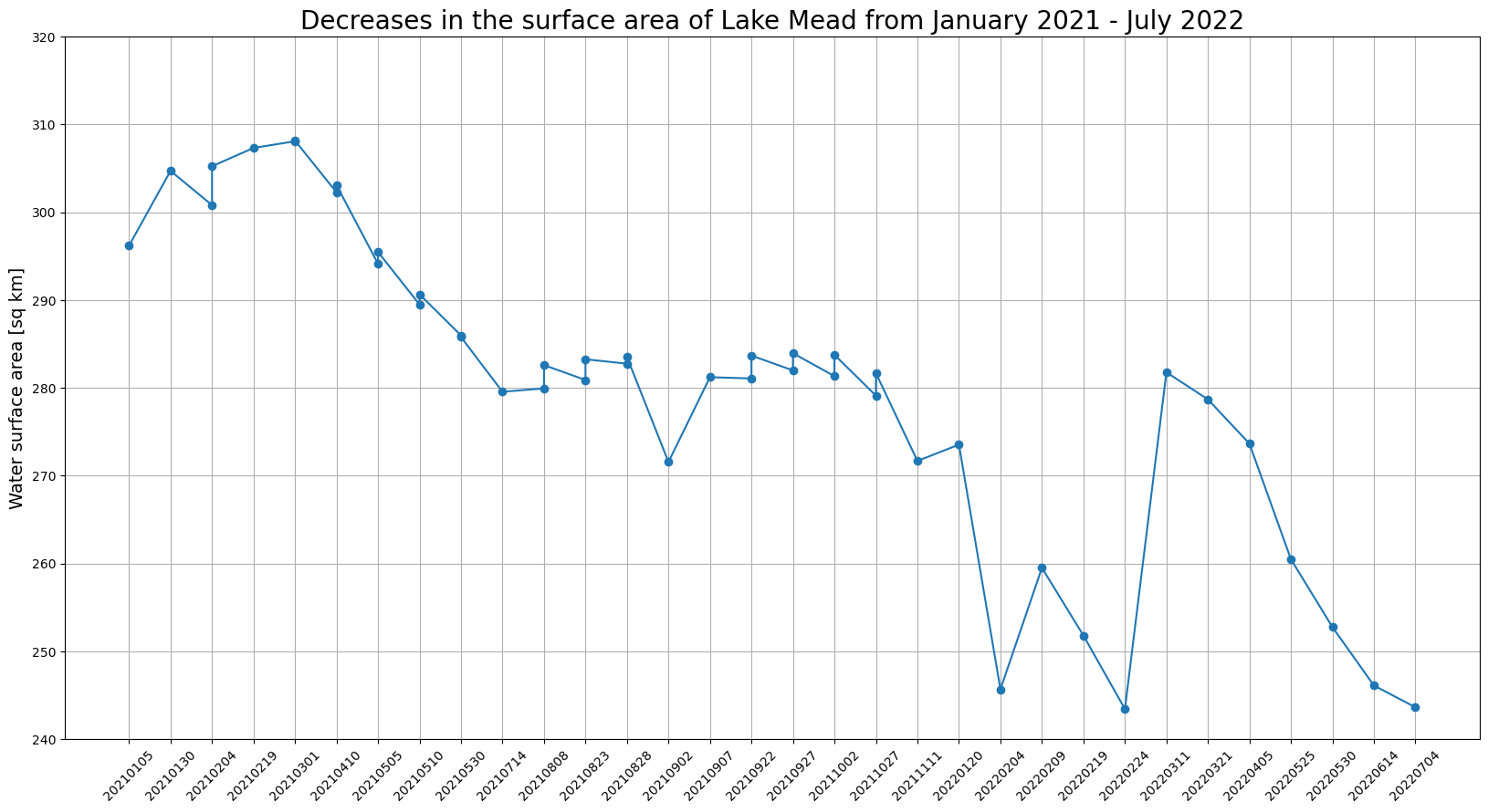
import os
from glob import glob
import cv2
import numpy as np
import tifffile
import matplotlib.pyplot as plt
from urllib.parse import urlparse
from botocore import UNSIGNED
from botocore.config import Config

# Download land cover masks
mask_dir = "./masks/lake_mead"
os.makedirs(mask_dir, exist_ok=True)
image_paths = []
for s3_object in s3_bucket.objects.filter(Prefix=prefix).all():
    path, filename = os.path.split(s3_object.key)
    if "output" in path:
        mask_name = mask_dir + "/" + filename
        s3_bucket.download_file(s3_object.key, mask_name)
        print("Downloaded mask: " + mask_name)

# Download source images for visualization
for tci_url in tci_urls:
    url_parts = urlparse(tci_url)
    img_id = url_parts.path.split("/")[-2]
    tci_download_path = image_dir + "/" + img_id + "_TCI.tif"
    cogs_bucket = session.resource(
        "s3", config=Config(signature_version=UNSIGNED, region_name="us-west-2")
    ).Bucket(url_parts.hostname.split(".")[0])
    cogs_bucket.download_file(url_parts.path[1:], tci_download_path)
    print("Downloaded image: " + img_id)

print("Downloads complete.")

image_files = glob("images/lake_mead/*.tif")
mask_files = glob("masks/lake_mead/*.tif")
image_files.sort(key=lambda x: x.split("SQA_")[1])
mask_files.sort(key=lambda x: x.split("SQA_")[1])
overlay_dir = "./masks/lake_mead_overlay"
os.makedirs(overlay_dir, exist_ok=True)
lake_areas = []
mask_dates = []

for image_file, mask_file in zip(image_files, mask_files):
    image_id = image_file.split("/")[-1].split("_TCI")[0]
    mask_id = mask_file.split("/")[-1].split(".tif")[0]
    mask_date = mask_id.split("_")[2]
    mask_dates.append(mask_date)
    assert image_id == mask_id
    image = tifffile.imread(image_file)
    image_ds = cv2.resize(image, (1830, 1830), interpolation=cv2.INTER_LINEAR)
    mask = tifffile.imread(mask_file)
    water_mask = np.isin(mask, [6]).astype(np.uint8)  # water has a class index 6
    lake_mask = water_mask[1000:, :1100]
    lake_area = lake_mask.sum() * 60 * 60 / (1000 * 1000)  # calculate the surface area
    lake_areas.append(lake_area)
    contour, _ = cv2.findContours(water_mask, cv2.RETR_TREE, cv2.CHAIN_APPROX_SIMPLE)
    combined = cv2.drawContours(image_ds, contour, -1, (255, 0, 0), 4)
    lake_crop = combined[1000:, :1100]
    cv2.putText(lake_crop, f"{mask_date}", (10,50), cv2.FONT_HERSHEY_SIMPLEX, 1.5, (0, 0, 0), 3, cv2.LINE_AA)
    cv2.putText(lake_crop, f"{lake_area} [sq km]", (10,100), cv2.FONT_HERSHEY_SIMPLEX, 1.5, (0, 0, 0), 3, cv2.LINE_AA)
    overlay_file = overlay_dir + '/' + mask_date + '.png'
    cv2.imwrite(overlay_file, cv2.cvtColor(lake_crop, cv2.COLOR_RGB2BGR))

# Plot water surface area vs. time.
plt.figure(figsize=(20,10))
plt.title('Lake Mead surface area for the 2021.02 - 2022.07 period.', fontsize=20)
plt.xticks(rotation=45)
plt.ylabel('Water surface area [sq km]', fontsize=14)
plt.plot(mask_dates, lake_areas, marker='o')
plt.grid('on')
plt.ylim(240, 320)
for i, v in enumerate(lake_areas):
    plt.text(i, v+2, "%d" %v, ha='center')
plt.show()

Using matplotlib, you can visualize the results with a graph. The graph shows that the surface area of Lake Mead decreased from January 2021–July 2022.