Evaluate your provisioned capacity for right-sized provisioning - Amazon DynamoDB
Services or capabilities described in Amazon Web Services documentation might vary by Region. To see the differences applicable to the China Regions, see Getting Started with Amazon Web Services in China (PDF).

Evaluate your provisioned capacity for right-sized provisioning

This section provides an overview of how to evaluate if you have right-sized provisioning on your DynamoDB tables. As your workload evolves, you should modify your operational procedures appropriately, especially when your DynamoDB table is configured in provisioned mode and you have the risk to over-provision or under-provision your tables.

The procedures described below require statistical information that should be captured from the DynamoDB tables that are supporting your production application. To understand your application behavior, you should define a period of time that is significant enough to capture the data seasonality from your application. For example, if your application shows weekly patterns, using a three week period should give you enough room for analysing application throughput needs.

If you don’t know where to start, use at least one month’s worth of data usage for the calculations below.

While evaluating capacity, DynamoDB tables can configure Read Capacity Units (RCUs) and Write Capacity Units (WCU) independently. If your tables have any Global Secondary Indexes (GSI) configured, you will need to specify the throughput that it will consume, which will be also independent from the RCUs and WCUs from the base table.

Note

Local Secondary Indexes (LSI) consume capacity from the base table.

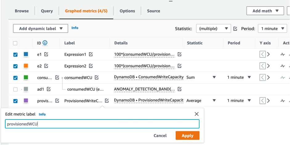
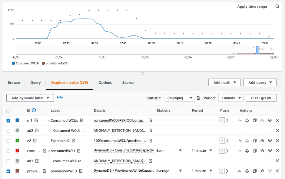
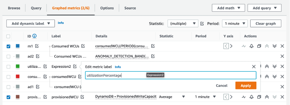
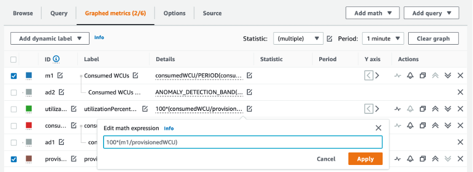
How to retrieve consumption metrics on your DynamoDB tables

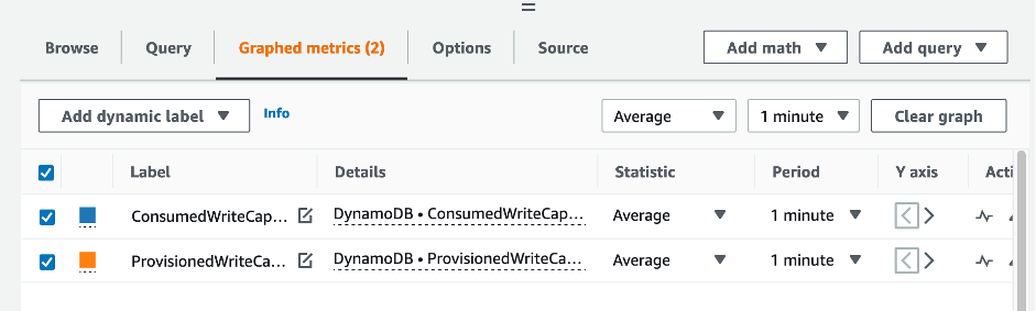
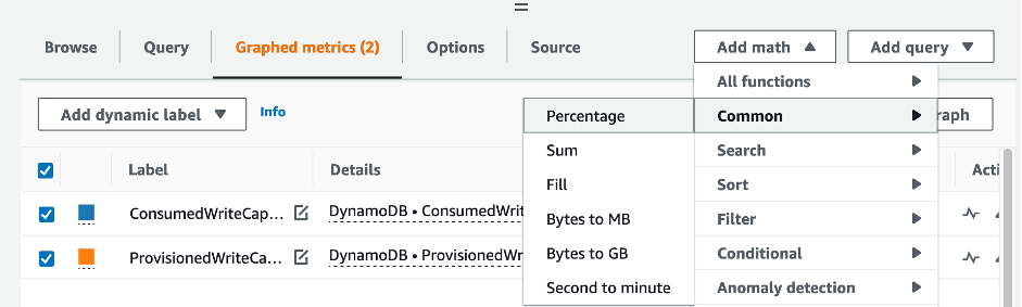
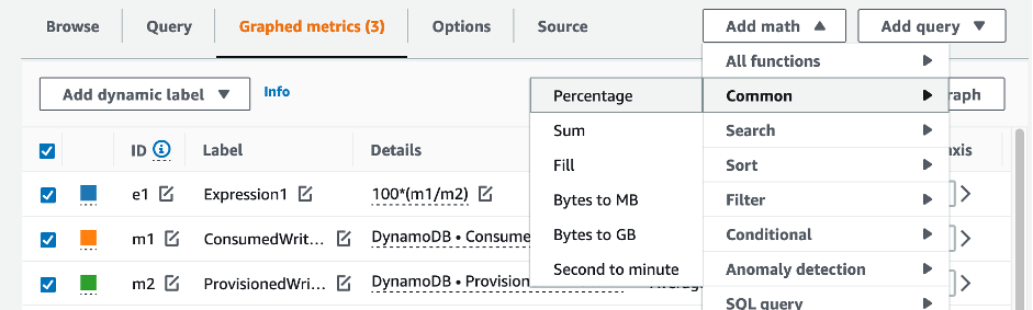
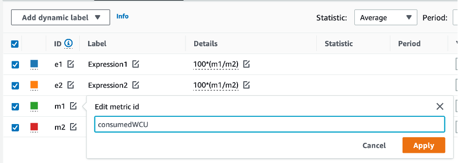
To evaluate the table and GSI capacity, monitor the following CloudWatch metrics and select the appropriate dimension to retrieve either table or GSI information:

Read Capacity Units Write Capacity Units

ConsumedReadCapacityUnits

ConsumedWriteCapacityUnits

ProvisionedReadCapacityUnits

ProvisionedWriteCapacityUnits

ReadThrottleEvents

WriteThrottleEvents

You can do this either through the Amazon CLI or the Amazon Web Services Management Console.

Amazon CLI

Before we retrieve the table consumption metrics, we'll need to start by capturing some historical data points using the CloudWatch API.

Start by creating two files: write-calc.json and read-calc.json. These files will represent the calculations for a table or GSI. You'll need to update some of the fields, as indicated in the table below, to match your environment.

Field Name Definition Example
<table-name> The name of the table that you will be analysing SampleTable
<period> The period of time that you will be using to evaluate the utilization target, based in seconds For a 1-hour period you should specify: 3600
<start-time> The beginning of your evaluation interval, specified in ISO8601 format 2022-02-21T23:00:00
<end-time> The end of your evaluation interval, specified in ISO8601 format 2022-02-22T06:00:00

The write calculations file will retrieve the number of WCU provisioned and consumed in the time period for the date range specified. It will also generate a utilization percentage that will be used for analysis. The full content of the write-calc.json file should look like this:

{ "MetricDataQueries": [ { "Id": "provisionedWCU", "MetricStat": { "Metric": { "Namespace": "AWS/DynamoDB", "MetricName": "ProvisionedWriteCapacityUnits", "Dimensions": [ { "Name": "TableName", "Value": "<table-name>" } ] }, "Period": <period>, "Stat": "Average" }, "Label": "Provisioned", "ReturnData": false }, { "Id": "consumedWCU", "MetricStat": { "Metric": { "Namespace": "AWS/DynamoDB", "MetricName": "ConsumedWriteCapacityUnits", "Dimensions": [ { "Name": "TableName", "Value": "<table-name>"" } ] }, "Period": <period>, "Stat": "Sum" }, "Label": "", "ReturnData": false }, { "Id": "m1", "Expression": "consumedWCU/PERIOD(consumedWCU)", "Label": "Consumed WCUs", "ReturnData": false }, { "Id": "utilizationPercentage", "Expression": "100*(m1/provisionedWCU)", "Label": "Utilization Percentage", "ReturnData": true } ], "StartTime": "<start-time>", "EndTime": "<ent-time>", "ScanBy": "TimestampDescending", "MaxDatapoints": 24 }

The read calculations file uses a similar file. This file will retrieve how many RCUs were provisioned and consumed during the time period for the date range specified. The contents of the read-calc.json file should look like this:

{ "MetricDataQueries": [ { "Id": "provisionedRCU", "MetricStat": { "Metric": { "Namespace": "AWS/DynamoDB", "MetricName": "ProvisionedReadCapacityUnits", "Dimensions": [ { "Name": "TableName", "Value": "<table-name>" } ] }, "Period": <period>, "Stat": "Average" }, "Label": "Provisioned", "ReturnData": false }, { "Id": "consumedRCU", "MetricStat": { "Metric": { "Namespace": "AWS/DynamoDB", "MetricName": "ConsumedReadCapacityUnits", "Dimensions": [ { "Name": "TableName", "Value": "<table-name>" } ] }, "Period": <period>, "Stat": "Sum" }, "Label": "", "ReturnData": false }, { "Id": "m1", "Expression": "consumedRCU/PERIOD(consumedRCU)", "Label": "Consumed RCUs", "ReturnData": false }, { "Id": "utilizationPercentage", "Expression": "100*(m1/provisionedRCU)", "Label": "Utilization Percentage", "ReturnData": true } ], "StartTime": "<start-time>", "EndTime": "<end-time>", "ScanBy": "TimestampDescending", "MaxDatapoints": 24 }

One you've created the files, you can start retrieving utilization data.

  1. To retreive the write utilization data, issue the following command:

    aws cloudwatch get-metric-data --cli-input-json file://write-calc.json
  2. To retreive the read utilization data, issue the following command:

    aws cloudwatch get-metric-data --cli-input-json file://read-calc.json

The result for both queries will be a series of data points in JSON format that will be used for analysis. Your result will depend on the number of data points you specified, the period, and your own specific workload data. It could look something like this:

{ "MetricDataResults": [ { "Id": "utilizationPercentage", "Label": "Utilization Percentage", "Timestamps": [ "2022-02-22T05:00:00+00:00", "2022-02-22T04:00:00+00:00", "2022-02-22T03:00:00+00:00", "2022-02-22T02:00:00+00:00", "2022-02-22T01:00:00+00:00", "2022-02-22T00:00:00+00:00", "2022-02-21T23:00:00+00:00" ], "Values": [ 91.55364583333333, 55.066631944444445, 2.6114930555555556, 24.9496875, 40.94725694444445, 25.61819444444444, 0.0 ], "StatusCode": "Complete" } ], "Messages": [] }
Note

If you specify a short period and a long time range, you might need to modify the MaxDatapoints which is by default set to 24 in the script. This represents one data point per hour and 24 per day.

Amazon Web Services Management Console
  1. Log into the Amazon Web Services Management Console and navigate to the CloudWatch service page at Getting Started with the Amazon Web Services Management Console. Select the appropriate Amazon region if necessary.

  2. Locate the Metrics section on the left navigation bar and select All metrics.

  3. This will open a dashboard with two panels. The top panel will show you the grapic, and the bottom panel will have the metrics you want to graph. Select the DynamoDB panel.

  4. Select the Table Metrics category from the sub panels. This will show you the tables in your current Region.

  5. Identify your table name by scrolling down the menu and selecting the write operation metrics: ConsumedWriteCapacityUnits and ProvisionedWriteCapacityUnits

    Note

    This example talks about write operation metrics, but you can also use these steps to graph the read operation metrics.

  6. Select the Graphed metrics (2) tab to modify the formulas. By default CloudWatch will select the statistical function Average for the graphs.

  7. While having both graphed metrics selected (the checkbox on the left) select the menu Add math, followed by Common, and then select the Percentage function. Repeat the procedure twice.

    First time selecting the Percentage function:

    Second time selecting the Percentage function:

  8. At this point you should have four metrics in the bottom menu. Let’s work on the ConsumedWriteCapacityUnits calculation. To be consistent, we need to match the names for the ones we used in the Amazon CLI section. Click on the m1 ID and change this value to consumedWCU.

  9. Change the statistic from Average to Sum. This action will automatically create another metric called ANOMALY_DETECTION_BAND. For the scope of this procedure, let's can ignore it by removing the checkbox on the newly generated ad1 metric.

  10. Repeat step 8 to rename the m2 ID to provisionedWCU. Leave the statistic set to Average.

  11. Select the Expression1 label and update the value to m1 and the label to Consumed WCUs.

    Note

    Make sure you have only selected m1 (checkbox on the left) and provisionedWCU to properly visualize the data. Update the formula by clicking in Details and changing the formula to consumedWCU/PERIOD(consumedWCU). This step might also generate another ANOMALY_DETECTION_BAND metric, but for the scope of this procedure we can ignore it.

  12. You should have now have two graphics: one that indicates your provisioned WCUs on the table and another that indicates the consumed WCUs. The shape of the graphic might be different from the one below, but you can use it as reference:

  13. Update the percentage formula by selecting the Expression2 graphic (e2). Rename the labels and IDs to utilizationPercentage. Rename the formula to match 100*(m1/provisionedWCU).

  14. Remove the checkbox from all the metrics but utilizationPercentage to visualize your utilization patterns. The default interval is set to 1 minute, but feel free to modify it as you need.

Here is view of a longer period of time as well as a bigger period of 1 hour. You can see there are some intervals where the utilization was higher than 100%, but this particular workload has longer intervals with zero utilization.

At this point, you might have different results from the pictures in this example. It all depends on the data from your workload. Intervals with more than 100% utilization are prone to throttling events. DynamoDB offers burst capacity, but as soon as the burst capacity is done anything above 100% will be throttled.

How to identify under-provisioned DynamoDB tables

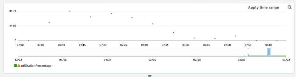
For most workloads, a table is considered under-provisioned when it constantly consumes more than 80% of their provisioned capacity.

Burst capacity is a DynamoDB feature that allow customers to temporarily consume more RCUs/WCUs than originally provisioned (more than the per-second provisioned throughput that was defined in the table). The burst capacity was created to absorb sudden increases in traffic due to special events or usage spikes. This burst capacity doesn’t last forever. As soon as the unused RCUs and WCUs are depleted, you will get throttled if you try to consume more capacity than provisioned. When your application traffic is getting close to the 80% utilization rate, your risk of throttling is significantly higher.

The 80% utilization rate rule varies from the seasonality of your data and your traffic growth. Consider the following scenarios:

  • If your traffic has been stable at ~90% utilization rate for the last 12 months, your table has just the right capacity

  • If your application traffic is growing at a rate of 8% monthly in less than 3 months, you will arrive at 100%

  • If your application traffic is growing at a rate of 5% in a little more than 4 months, you will still arrive at 100%

The results from the queries above provide a picture of your utilization rate. Use them as a guide to further evaluate other metrics that can help you choose to increase your table capacity as required (for example: a monthly or weekly growth rate). Work with your operations team to define what is a good percentage for your workload and your tables.

There are special scenarios where the data is skewed when we analyse it on a daily or weekly basis. For example, with seasonal applications that have spikes in usage during working hours (but then drops to almost zero outside of working hours), you could benefit by scheduling auto scaling where you specify the hours of the day (and the days of the week) to increase the provisioned capacity and when to reduce it. Instead of aiming for higher capacity so you can cover the busy hours, you can also benefit from DynamoDB table auto scaling configurations if your seasonality is less pronounced.

Note

When you create a DynamoDB auto scaling configuration for your base table, remember to include another configuration for any GSI that is associated with the table.

How to identify over-provisioned DynamoDB tables

The query results obtained from the scripts above provide the data points required to perform some initial analysis. If your data set presents values lower than 20% utilization for several intervals, your table might be over-provisioned. To further define if you need to reduce the number of WCUs and RCUS, you should revisit the other readings in the intervals.

When your tables contain several low usage intervals, you can really benefit from using auto scaling policies, either by scheduling auto scaling or just configuring the default auto scaling policies for the table that are based on utilization.

If you have a workload with low utilization to high throttle ratio (Max(ThrottleEvents)/Min(ThrottleEvents) in the interval), this could happen when you have a very spiky workload where traffic increases a lot during some days (or hours), but in general the traffic is consistently low. In these scenarios it might be beneficial to use scheduled auto scaling.