Transform Data
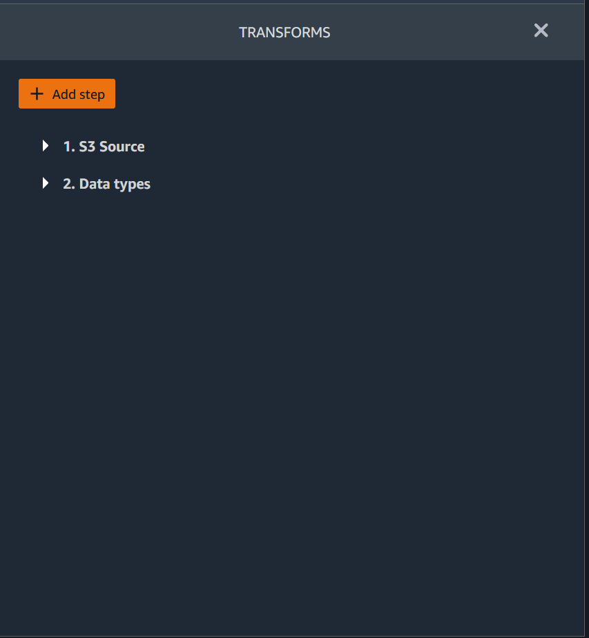
Amazon SageMaker Data Wrangler provides numerous ML data transforms to streamline cleaning, transforming, and featurizing your data. When you add a transform, it adds a step to the data flow. Each transform you add modifies your dataset and produces a new dataframe. All subsequent transforms apply to the resulting dataframe.
Data Wrangler includes built-in transforms, which you can use to transform columns without any code. You can also add custom transformations using PySpark, Python (User-Defined Function), pandas, and PySpark SQL. Some transforms operate in place, while others create a new output column in your dataset.
You can apply transforms to multiple columns at once. For example, you can delete multiple columns in a single step.
You can apply the Process numeric and Handle missing transforms only to a single column.
Use this page to learn more about these built-in and custom transforms.
Transform UI
Most of the built-in transforms are located in the Prepare tab of the Data Wrangler UI. You can access the join and concatenate transforms through the data flow view. Use the following table to preview these two views.

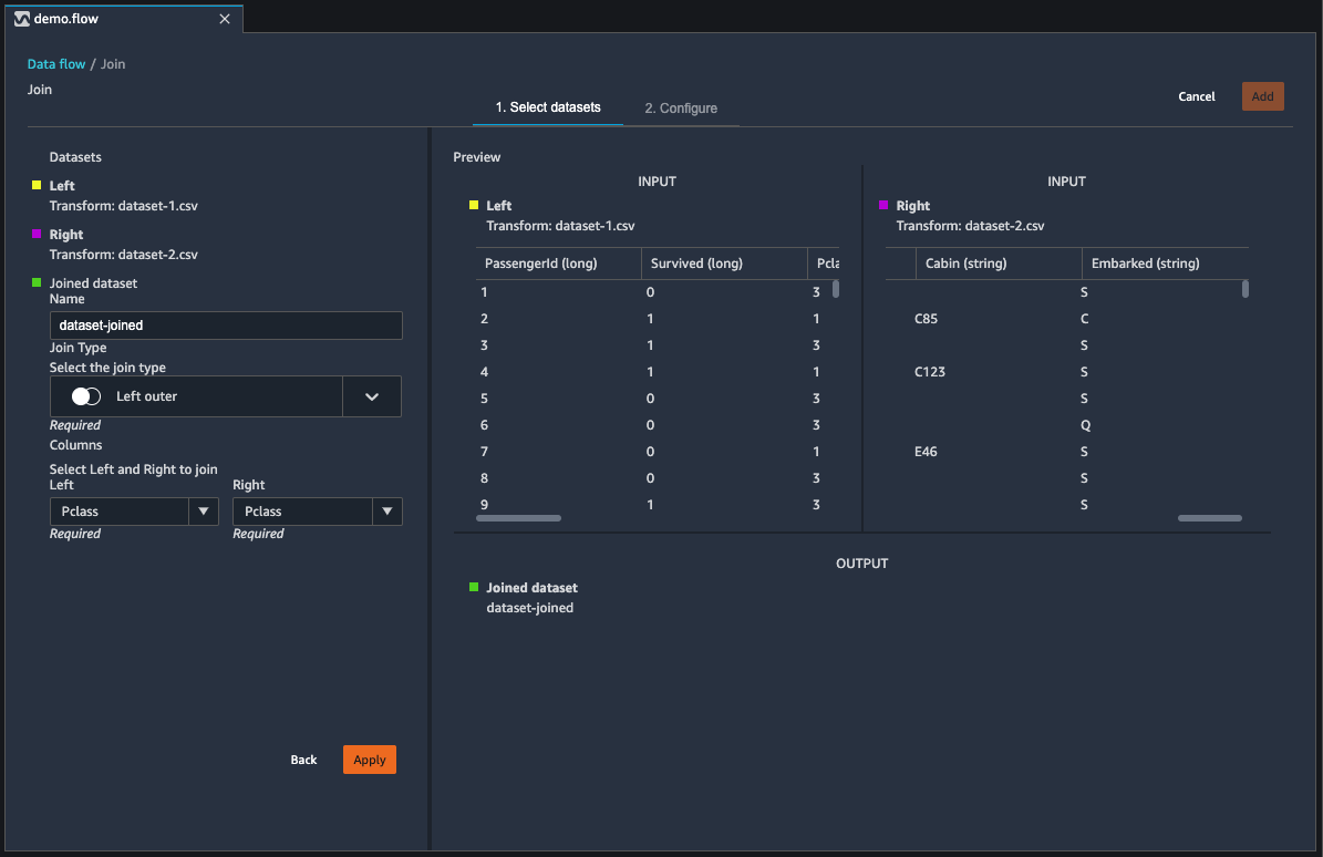
Join Datasets
You join dataframes directly in your data flow. When you join two datasets, the resulting joined dataset appears in your flow. The following join types are supported by Data Wrangler.
-
Left Outer – Include all rows from the left table. If the value for the column joined on a left table row does not match any right table row values, that row contains null values for all right table columns in the joined table.
-
Left Anti – Include rows from the left table that do not contain values in the right table for the joined column.
-
Left semi – Include a single row from the left table for all identical rows that satisfy the criteria in the join statement. This excludes duplicate rows from the left table that match the criteria of the join.
-
Right Outer – Include all rows from the right table. If the value for the joined column in a right table row does not match any left table row values, that row contains null values for all left table columns in the joined table.
-
Inner – Include rows from left and right tables that contain matching values in the joined column.
-
Full Outer – Include all rows from the left and right tables. If the row value for the joined column in either table does not match, separate rows are created in the joined table. If a row doesn’t contain a value for a column in the joined table, null is inserted for that column.
-
Cartesian Cross – Include rows which combine each row from the first table with each row from the second table. This is a Cartesian product
of rows from tables in the join. The result of this product is the size of the left table times the size of the right table. Therefore, we recommend caution in using this join between very large datasets.
Use the following procedure to join two dataframes.
-
Select + next to the left dataframe that you want to join. The first dataframe you select is always the left table in your join.
-
Choose Join.
-
Select the right dataframe. The second dataframe you select is always the right table in your join.
-
Choose Configure to configure your join.
-
Give your joined dataset a name using the Name field.
-
Select a Join type.
-
Select a column from the left and right tables to join.
-
Choose Apply to preview the joined dataset on the right.
-
To add the joined table to your data flow, choose Add.
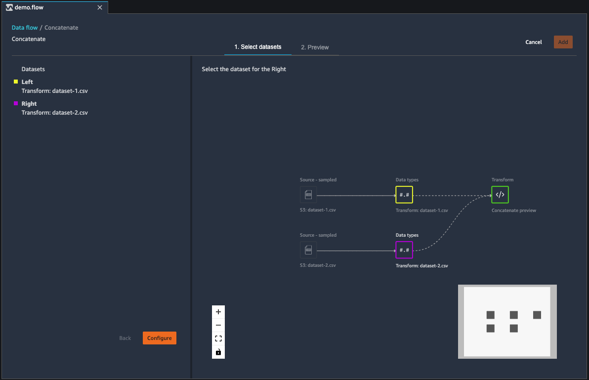
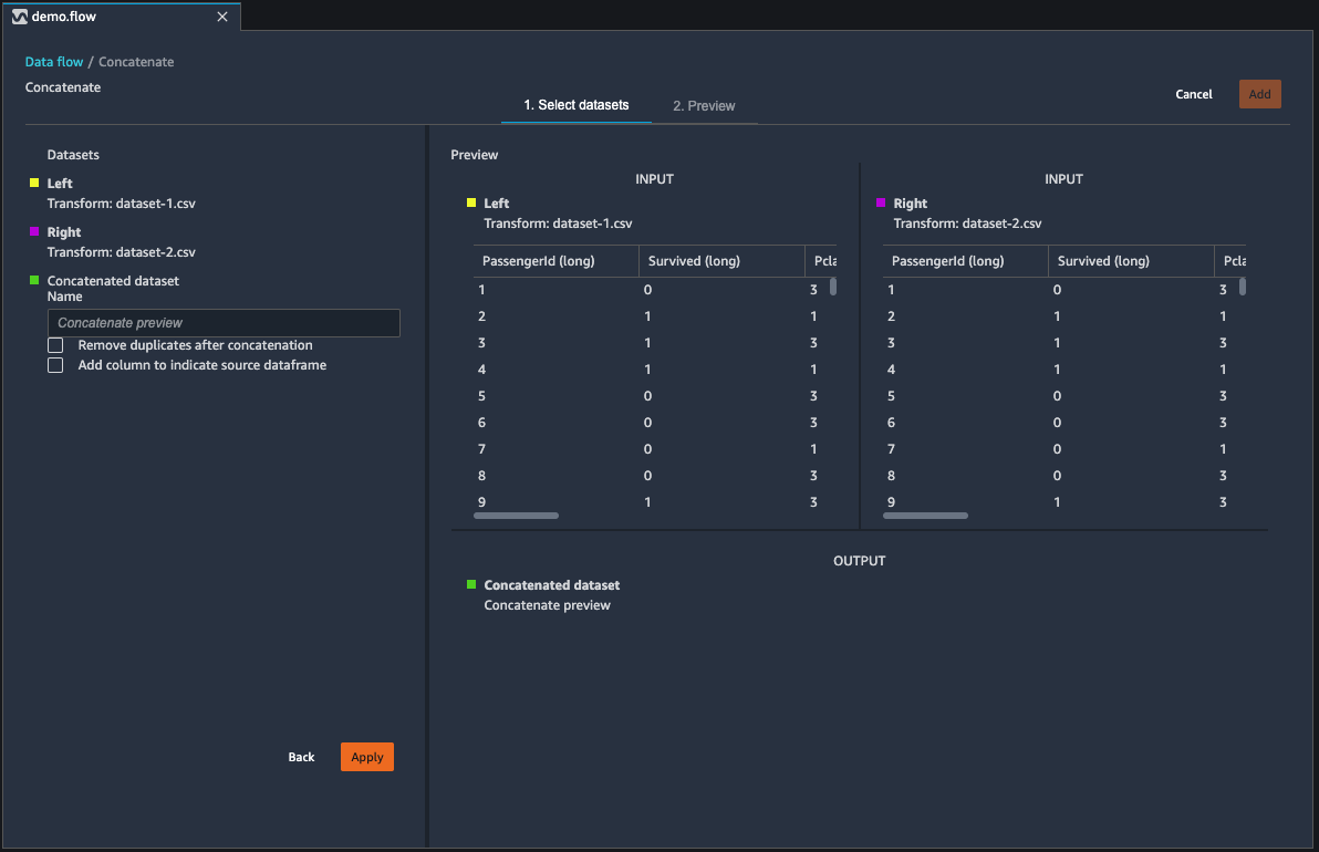
Concatenate Datasets
Concatenate two datasets:
-
Choose + next to the left dataframe that you want to concatenate. The first dataframe you select is always the left table in your concatenate.
-
Choose Concatenate.
-
Select the right dataframe. The second dataframe you select is always the right table in your concatenate.
-
Choose Configure to configure your concatenate.
-
Give your concatenated dataset a name using the Name field.
-
(Optional) Select the checkbox next to Remove duplicates after concatenation to remove duplicate columns.
-
(Optional) Select the checkbox next to Add column to indicate source dataframe if, for each column in the new dataset, you want to add an indicator of the column's source.
-
Choose Apply to preview the new dataset.
-
Choose Add to add the new dataset to your data flow.
Balance Data
You can balance the data for datasets with an underrepresented category. Balancing a dataset can help you create better models for binary classification.
Note
You can't balance datasets containing column vectors.
You can use the Balance data operation to balance your data using one of the following operators:
-
Random oversampling – Randomly duplicates samples in the minority category. For example, if you're trying to detect fraud, you might only have cases of fraud in 10% of your data. For an equal proportion of fraudulent and non-fraudulent cases, this operator randomly duplicates fraud cases within the dataset 8 times.
-
Random undersampling – Roughly equivalent to random oversampling. Randomly removes samples from the overrepresented category to get the proportion of samples that you desire.
-
Synthetic Minority Oversampling Technique (SMOTE) – Uses samples from the underrepresented category to interpolate new synthetic minority samples. For more information about SMOTE, see the following description.
You can use all transforms for datasets containing both numeric and non-numeric features. SMOTE interpolates values by using neighboring samples. Data Wrangler uses the R-squared distance to determine the neighborhood to interpolate the additional samples. Data Wrangler only uses numeric features to calculate the distances between samples in the underrepresented group.
For two real samples in the underrepresented group, Data Wrangler interpolates the numeric features by using a weighted average. It randomly assigns weights to those samples in the range of [0, 1]. For numeric features, Data Wrangler interpolates samples using a weighted average of the samples. For samples A and B, Data Wrangler could randomly assign a weight of 0.7 to A and 0.3 to B. The interpolated sample has a value of 0.7A + 0.3B.
Data Wrangler interpolates non-numeric features by copying from either of the interpolated real samples. It copies the samples with a probability that it randomly assigns to each sample. For samples A and B, it can assign probabilities 0.8 to A and 0.2 to B. For the probabilities it assigned, it copies A 80% of the time.
Custom Transforms
The Custom Transforms group allows you to use Python
(User-Defined Function), PySpark, pandas, or PySpark (SQL) to define custom
transformations. For all three options, you use the variable df to access
the dataframe to which you want to apply the transform. To apply your custom code to your dataframe, assign the dataframe with the transformations that you've made to the df variable.
If you're not using Python
(User-Defined Function), you don't need to include a return statement. Choose
Preview to preview the result of the custom transform. Choose
Add to add the custom transform to your list of
Previous steps.
You can import the popular libraries with an import statement in the
custom transform code block, such as the following:
-
NumPy version 1.19.0
-
scikit-learn version 0.23.2
-
SciPy version 1.5.4
-
pandas version 1.0.3
-
PySpark version 3.0.0
Important
Custom transform doesn't support columns with spaces or
special characters in the name. We recommend that you specify column names that only
have alphanumeric characters and underscores. You can use the Rename
column transform in the Manage columns transform
group to remove spaces from a column's name. You can also add a Python
(Pandas)
Custom transform similar to the following to remove spaces from
multiple columns in a single step. This example changes columns named A
column and B column to A_column and
B_column respectively.
df.rename(columns={"A column": "A_column", "B column": "B_column"})
If you include print statements in the code block, the result appears when you select Preview. You can resize the custom code transformer panel. Resizing the panel provides more space to write code. The following image shows the resizing of the panel.
The following sections provide additional context and examples for writing custom transform code.
Python (User-Defined Function)
The Python function gives you the ability to write custom transformations without needing to know Apache Spark or pandas. Data Wrangler is optimized to run your custom code quickly. You get similar performance using custom Python code and an Apache Spark plugin.
To use the Python (User-Defined Function) code block, you specify the following:
-
Input column – The input column where you're applying the transform.
-
Mode – The scripting mode, either pandas or Python.
-
Return type – The data type of the value that you're returning.
Using the pandas mode gives better performance. The Python mode makes it easier for you to write transformations by using pure Python functions.
The following video shows an example of how to use custom code to create a
transformation. It uses the
Titanic dataset
PySpark
The following example extracts date and time from a timestamp.
from pyspark.sql.functions import from_unixtime, to_date, date_format
df = df.withColumn('DATE_TIME', from_unixtime('TIMESTAMP'))
df = df.withColumn( 'EVENT_DATE', to_date('DATE_TIME')).withColumn(
'EVENT_TIME', date_format('DATE_TIME', 'HH:mm:ss'))
pandas
The following example provides an overview of the dataframe to which you are adding transforms.
df.info()
PySpark (SQL)
The following example creates a new dataframe with four columns: name, fare, pclass, survived.
SELECT name, fare, pclass, survived FROM df
If you don’t know how to use PySpark, you can use custom code snippets to help you get started.
Data Wrangler has a searchable collection of code snippets. You can use to code snippets to perform tasks such as dropping columns, grouping by columns, or modelling.
To use a code snippet, choose Search example snippets and specify a query in the search bar. The text you specify in the query doesn’t have to match the name of the code snippet exactly.
The following example shows a Drop duplicate rows code snippet that can delete rows with similar data in your dataset. You can find the code snippet by searching for one of the following:
-
Duplicates
-
Identical
-
Remove
The following snippet has comments to help you understand the changes that you need to make. For most snippets, you must specify the column names of your dataset in the code.
# Specify the subset of columns
# all rows having identical values in these columns will be dropped

subset = ["col1", "col2", "col3"]
df = df.dropDuplicates(subset)

# to drop the full-duplicate rows run
# df = df.dropDuplicates()
To use a snippet, copy and paste its content into the Custom transform field. You can copy and paste multiple code snippets into the custom transform field.
Custom Formula
Use Custom formula to define a new column using a Spark SQL expression to query data in the current dataframe. The query must use the conventions of Spark SQL expressions.
Important
Custom formula doesn't support columns with spaces or special
characters in the name. We recommend that you specify column names that only have
alphanumeric characters and underscores. You can use the Rename
column transform in the Manage columns transform
group to remove spaces from a column's name. You can also add a Python
(Pandas)
Custom transform similar to the following to remove spaces from
multiple columns in a single step. This example changes columns named A
column and B column to A_column and
B_column respectively.
df.rename(columns={"A column": "A_column", "B column": "B_column"})
You can use this transform to perform operations on columns, referencing the columns by name. For example, assuming the current dataframe contains columns named col_a and col_b, you can use the following operation to produce an Output column that is the product of these two columns with the following code:
col_a * col_b
Other common operations include the following, assuming a dataframe contains
col_a and col_b columns:
-
Concatenate two columns:
concat(col_a, col_b) -
Add two columns:
col_a + col_b -
Subtract two columns:
col_a - col_b -
Divide two columns:
col_a / col_b -
Take the absolute value of a column:
abs(col_a)
For more information, see the Spark documentation
Reduce Dimensionality within a Dataset
Reduce the dimensionality in your data by using Principal Component Analysis (PCA). The dimensionality of your dataset corresponds to the number of features. When you use dimensionality reduction in Data Wrangler, you get a new set of features called components. Each component accounts for some variability in the data.
The first component accounts for the largest amount of variation in the data. The second component accounts for the second largest amount of variation in the data, and so on.
You can use dimensionality reduction to reduce the size of the data sets that you use to train models. Instead of using the features in your dataset, you can use the principal components instead.
To perform PCA, Data Wrangler creates axes for your data. An axis is an affine combination of columns in your dataset. The first principal component is the value on the axis that has the largest amount of variance. The second principal component is the value on the axis that has the second largest amount of variance. The nth principal component is the value on the axis that has the nth largest amount of variance.
You can configure the number of principal components that Data Wrangler returns. You can either specify the number of principal components directly or you can specify the variance threshold percentage. Each principal component explains an amount of variance in the data. For example, you might have a principal component with a value of 0.5. The component would explain 50% of the variation in the data. When you specify a variance threshold percentage, Data Wrangler returns the smallest number of components that meet the percentage that you specify.
The following are example principal components with the amount of variance that they explain in the data.
-
Component 1 – 0.5
-
Component 2 – 0.45
-
Component 3 – 0.05
If you specify a variance threshold percentage of 94 or 95, Data Wrangler returns Component 1 and Component 2. If you specify a variance threshold percentage of 96, Data Wrangler returns all three principal components.
You can use the following procedure to run PCA on your dataset.
To run PCA on your dataset, do the following.
-
Open your Data Wrangler data flow.
-
Choose the +, and select Add transform.
-
Choose Add step.
-
Choose Dimensionality Reduction.
-
For Input Columns, choose the features that you're reducing into the principal components.
-
(Optional) For Number of principal components, choose the number of principal components that Data Wrangler returns in your dataset. If specify a value for the field, you can't specify a value for Variance threshold percentage.
-
(Optional) For Variance threshold percentage, specify the percentage of variation in the data that you want explained by the principal components. Data Wrangler uses the default value of
95if you don't specify a value for the variance threshold. You can't specify a variance threshold percentage if you've specified a value for Number of principal components. -
(Optional) Deselect Center to not use the mean of the columns as the center of the data. By default, Data Wrangler centers the data with the mean before scaling.
-
(Optional) Deselect Scale to not scale the data with the unit standard deviation.
-
(Optional) Choose Columns to output the components to separate columns. Choose Vector to output the components as a single vector.
-
(Optional) For Output column, specify a name for an output column. If you're outputting the components to separate columns, the name that you specify is a prefix. If you're outputting the components to a vector, the name that you specify is the name of the vector column.
-
(Optional) Select Keep input columns. We don't recommend selecting this option if you plan on only using the principal components to train your model.
-
Choose Preview.
-
Choose Add.
Encode Categorical
Categorical data is usually composed of a finite number of categories, where each category is represented with a string. For example, if you have a table of customer data, a column that indicates the country a person lives in is categorical. The categories would be Afghanistan, Albania, Algeria, and so on. Categorical data can be nominal or ordinal. Ordinal categories have an inherent order, and nominal categories do not. The highest degree obtained (High school, Bachelors, Masters, and so on) is an example of ordinal categories.
Encoding categorical data is the process of creating a numerical representation for
categories. For example, if your categories are Dog
and Cat, you may encode this information into two
vectors, [1,0] to represent Dog, and
[0,1] to represent Cat.
When you encode ordinal categories, you may need to translate the natural order of
categories into your encoding. For example, you can represent the highest degree
obtained with the following map: {"High school": 1, "Bachelors": 2,
"Masters":3}.
Use categorical encoding to encode categorical data that is in string format into arrays of integers.
The Data Wrangler categorical encoders create encodings for all categories that exist in a column at the time the step is defined. If new categories have been added to a column when you start a Data Wrangler job to process your dataset at time t, and this column was the input for a Data Wrangler categorical encoding transform at time t-1, these new categories are considered missing in the Data Wrangler job. The option you select for Invalid handling strategy is applied to these missing values. Examples of when this can occur are:
-
When you use a .flow file to create a Data Wrangler job to process a dataset that was updated after the creation of the data flow. For example, you may use a data flow to regularly process sales data each month. If that sales data is updated weekly, new categories may be introduced into columns for which an encode categorical step is defined.
-
When you select Sampling when you import your dataset, some categories may be left out of the sample.
In these situations, these new categories are considered missing values in the Data Wrangler job.
You can choose from and configure an ordinal and a one-hot encode. Use the following sections to learn more about these options.
Both transforms create a new column named Output column name. You specify the output format of this column with Output style:
-
Select Vector to produce a single column with a sparse vector.
-
Select Columns to create a column for every category with an indicator variable for whether the text in the original column contains a value that is equal to that category.
Ordinal Encode
Select Ordinal encode to encode categories into an integer between 0 and the total number of categories in the Input column you select.
Invalid handing strategy: Select a method to handle invalid or missing values.
-
Choose Skip if you want to omit the rows with missing values.
-
Choose Keep to retain missing values as the last category.
-
Choose Error if you want Data Wrangler to throw an error if missing values are encountered in the Input column.
-
Choose Replace with NaN to replace missing with NaN. This option is recommended if your ML algorithm can handle missing values. Otherwise, the first three options in this list may produce better results.
One-Hot Encode
Select One-hot encode for Transform to use one-hot encoding. Configure this transform using the following:
-
Drop last category: If
True, the last category does not have a corresponding index in the one-hot encoding. When missing values are possible, a missing category is always the last one and setting this toTruemeans that a missing value results in an all zero vector. -
Invalid handing strategy: Select a method to handle invalid or missing values.
-
Choose Skip if you want to omit the rows with missing values.
-
Choose Keep to retain missing values as the last category.
-
Choose Error if you want Data Wrangler to throw an error if missing values are encountered in the Input column.
-
-
Is input ordinal encoded: Select this option if the input vector contains ordinal encoded data. This option requires that input data contain non-negative integers. If True, input i is encoded as a vector with a non-zero in the ith location.
Similarity encode
Use similarity encoding when you have the following:
-
A large number of categorical variables
-
Noisy data
The similarity encoder creates embeddings for columns with categorical data. An embedding is a mapping of discrete objects, such as words, to vectors of real numbers. It encodes similar strings to vectors containing similar values. For example, it creates very similar encodings for "California" and "Calfornia".
Data Wrangler converts each category in your dataset into a set of tokens using a 3-gram tokenizer. It converts the tokens into an embedding using min-hash encoding.
The following example shows how the similarity encoder creates vectors from strings.
The similarity encodings that Data Wrangler creates:
-
Have low dimensionality
-
Are scalable to a large number of categories
-
Are robust and resistant to noise
For the preceding reasons, similarity encoding is more versatile than one-hot encoding.
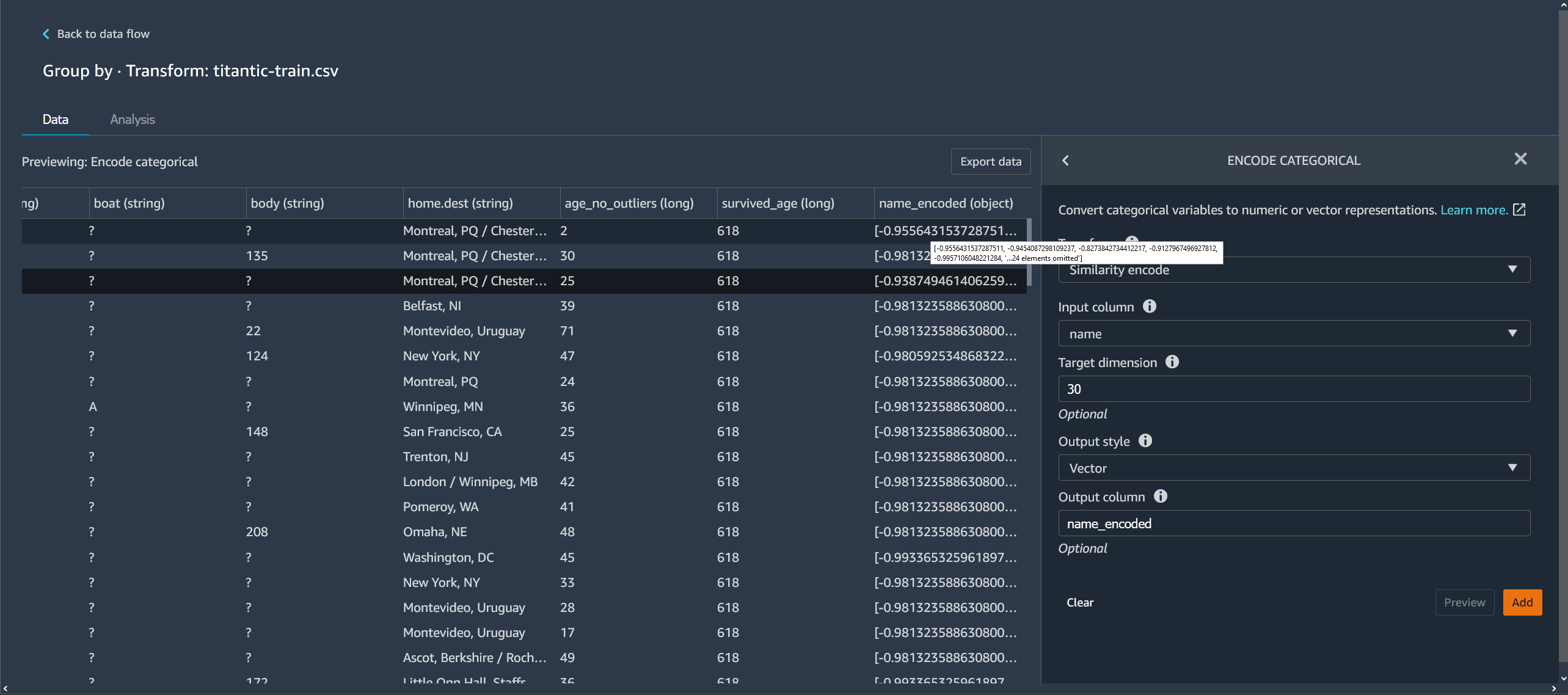
To add the similarity encoding transform to your dataset, use the following procedure.
To use similarity encoding, do the following.
-
Sign in to the Amazon SageMaker AI Console
. -
Choose Open Studio Classic.
-
Choose Launch app.
-
Choose Studio.
-
Specify your data flow.
-
Choose a step with a transformation.
-
Choose Add step.
-
Choose Encode categorical.
-
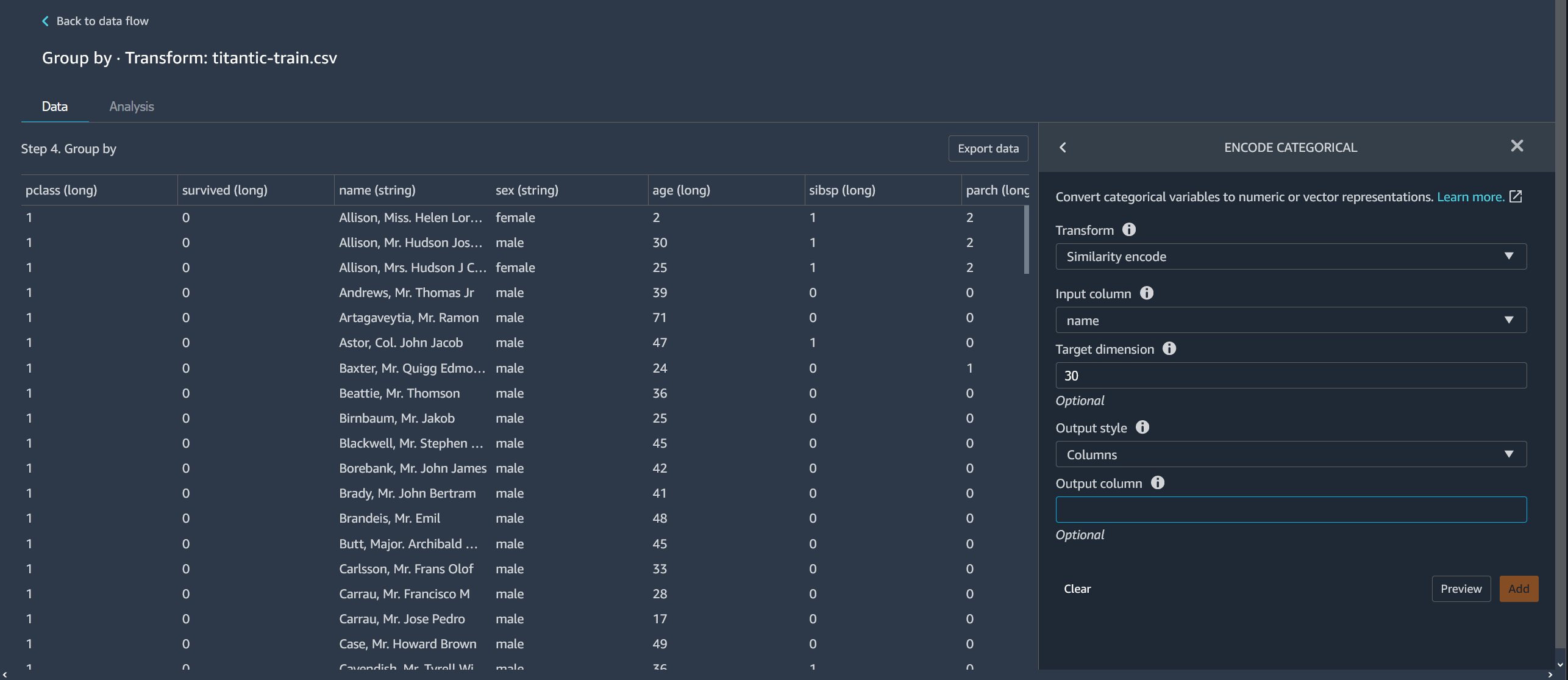
Specify the following:
-
Transform – Similarity encode
-
Input column – The column containing the categorical data that you're encoding.
-
Target dimension – (Optional) The dimension of the categorical embedding vector. The default value is 30. We recommend using a larger target dimension if you have a large dataset with many categories.
-
Output style – Choose Vector for a single vector with all of the encoded values. Choose Column to have the encoded values in separate columns.
-
Output column – (Optional) The name of the output column for a vector encoded output. For a column-encoded output, this is the prefix of the column names followed by listed number.
-
Featurize Text
Use the Featurize Text transform group to inspect string-typed columns and use text embedding to featurize these columns.
This feature group contains two features, Character statistics and Vectorize. Use the following sections to learn more about these transforms. For both options, the Input column must contain text data (string type).
Character Statistics
Use Character statistics to generate statistics for each row in a column containing text data.
This transform computes the following ratios and counts for each row, and creates a new column to report the result. The new column is named using the input column name as a prefix and a suffix that is specific to the ratio or count.
-
Number of words: The total number of words in that row. The suffix for this output column is
-stats_word_count. -
Number of characters: The total number of characters in that row. The suffix for this output column is
-stats_char_count. -
Ratio of upper: The number of uppercase characters, from A to Z, divided by all characters in the column. The suffix for this output column is
-stats_capital_ratio. -
Ratio of lower: The number of lowercase characters, from a to z, divided by all characters in the column. The suffix for this output column is
-stats_lower_ratio. -
Ratio of digits: The ratio of digits in a single row over the sum of digits in the input column. The suffix for this output column is
-stats_digit_ratio. -
Special characters ratio: The ratio of non-alphanumeric (characters like #$&%:@) characters to over the sum of all characters in the input column. The suffix for this output column is
-stats_special_ratio.
Vectorize
Text embedding involves mapping words or phrases from a vocabulary to vectors of real numbers. Use the Data Wrangler text embedding transform to tokenize and vectorize text data into term frequency–inverse document frequency (TF-IDF) vectors.
When TF-IDF is calculated for a column of text data, each word in each sentence is converted to a real number that represents its semantic importance. Higher numbers are associated with less frequent words, which tend to be more meaningful.
When you define a Vectorize transform step, Data Wrangler uses the data in your dataset to define the count vectorizer and TF-IDF methods . Running a Data Wrangler job uses these same methods.
You configure this transform using the following:
-
Output column name: This transform creates a new column with the text embedding. Use this field to specify a name for this output column.
-
Tokenizer: A tokenizer converts the sentence into a list of words, or tokens.
Choose Standard to use a tokenizer that splits by white space and converts each word to lowercase. For example,
"Good
                            dog"
is tokenized to["good","dog"].Choose Custom to use a customized tokenizer. If you choose Custom, you can use the following fields to configure the tokenizer:
-
Minimum token length: The minimum length, in characters, for a token to be valid. Defaults to
1. For example, if you specify3for minimum token length, words likea, at, inare dropped from the tokenized sentence. -
Should regex split on gaps: If selected, regex splits on gaps. Otherwise, it matches tokens. Defaults to
True. -
Regex pattern: Regex pattern that defines the tokenization process. Defaults to
' \\ s+'. -
To lowercase: If chosen, Data Wrangler converts all characters to lowercase before tokenization. Defaults to
True.
To learn more, see the Spark documentation on Tokenizer
. -
-
Vectorizer: The vectorizer converts the list of tokens into a sparse numeric vector. Each token corresponds to an index in the vector and a non-zero indicates the existence of the token in the input sentence. You can choose from two vectorizer options, Count and Hashing.
-
Count vectorize allows customizations that filter infrequent or too common tokens. Count vectorize parameters include the following:
-
Minimum term frequency: In each row, terms (tokens) with smaller frequency are filtered. If you specify an integer, this is an absolute threshold (inclusive). If you specify a fraction between 0 (inclusive) and 1, the threshold is relative to the total term count. Defaults to
1. -
Minimum document frequency: Minimum number of rows in which a term (token) must appear to be included. If you specify an integer, this is an absolute threshold (inclusive). If you specify a fraction between 0 (inclusive) and 1, the threshold is relative to the total term count. Defaults to
1. -
Maximum document frequency: Maximum number of documents (rows) in which a term (token) can appear to be included. If you specify an integer, this is an absolute threshold (inclusive). If you specify a fraction between 0 (inclusive) and 1, the threshold is relative to the total term count. Defaults to
0.999. -
Maximum vocabulary size: Maximum size of the vocabulary. The vocabulary is made up of all terms (tokens) in all rows of the column. Defaults to
262144. -
Binary outputs: If selected, the vector outputs do not include the number of appearances of a term in a document, but rather are a binary indicator of its appearance. Defaults to
False.
To learn more about this option, see the Spark documentation on CountVectorizer
. -
-
Hashing is computationally faster. Hash vectorize parameters includes the following:
-
Number of features during hashing: A hash vectorizer maps tokens to a vector index according to their hash value. This feature determines the number of possible hash values. Large values result in fewer collisions between hash values but a higher dimension output vector.
To learn more about this option, see the Spark documentation on FeatureHasher
-
-
-
Apply IDF applies an IDF transformation, which multiplies the term frequency with the standard inverse document frequency used for TF-IDF embedding. IDF parameters include the following:
-
Minimum document frequency : Minimum number of documents (rows) in which a term (token) must appear to be included. If count_vectorize is the chosen vectorizer, we recommend that you keep the default value and only modify the min_doc_freq field in Count vectorize parameters. Defaults to
5.
-
-
Output format:The output format of each row.
-
Select Vector to produce a single column with a sparse vector.
-
Select Flattened to create a column for every category with an indicator variable for whether the text in the original column contains a value that is equal to that category. You can only choose flattened when Vectorizer is set as Count vectorizer.
-
Transform Time Series
In Data Wrangler, you can transform time series data. The values in a time series dataset are indexed to specific time. For example, a dataset that shows the number of customers in a store for each hour in a day is a time series dataset. The following table shows an example of a time series dataset.
Hourly number of customers in a store
| Number of customers | Time (hour) |
|---|---|
| 4 | 09:00 |
| 10 | 10:00 |
| 14 | 11:00 |
| 25 | 12:00 |
| 20 | 13:00 |
| 18 | 14:00 |
For the preceding table, the Number of Customers column contains the time series data. The time series data is indexed on the hourly data in the Time (hour) column.
You might need to perform a series of transformations on your data to get it in a format that you can use for your analysis. Use the Time series transform group to transform your time series data. For more information about the transformations that you can perform, see the following sections.
Topics
Group by a Time Series
You can use the group by operation to group time series data for specific values in a column.
For example, you have the following table that tracks the average daily electricity usage in a household.
Average daily household electricity usage
| Household ID | Daily timestamp | Electricity usage (kWh) | Number of household occupants |
|---|---|---|---|
| household_0 | 1/1/2020 | 30 | 2 |
| household_0 | 1/2/2020 | 40 | 2 |
| household_0 | 1/4/2020 | 35 | 3 |
| household_1 | 1/2/2020 | 45 | 3 |
| household_1 | 1/3/2020 | 55 | 4 |
If you choose to group by ID, you get the following table.
Electricity usage grouped by household ID
| Household ID | Electricity usage series (kWh) | Number of household occupants series |
|---|---|---|
| household_0 | [30, 40, 35] | [2, 2, 3] |
| household_1 | [45, 55] | [3, 4] |
Each entry in the time series sequence is ordered by the corresponding timestamp.
The first element of the sequence corresponds to the first timestamp of the series.
For household_0, 30 is the first value of the
Electricity Usage Series. The value of 30
corresponds to the first timestamp of 1/1/2020.
You can include the starting timestamp and ending timestamp. The following table shows how that information appears.
Electricity usage grouped by household ID
| Household ID | Electricity usage series (kWh) | Number of household occupants series | Start_time | End_time |
|---|---|---|---|---|
| household_0 | [30, 40, 35] | [2, 2, 3] | 1/1/2020 | 1/4/2020 |
| household_1 | [45, 55] | [3, 4] | 1/2/2020 | 1/3/2020 |
You can use the following procedure to group by a time series column.
-
Open your Data Wrangler data flow.
-
If you haven't imported your dataset, import it under the Import data tab.
-
In your data flow, under Data types, choose the +, and select Add transform.
-
Choose Add step.
-
Choose Time Series.
-
Under Transform, choose Group by.
-
Specify a column in Group by this column.
-
For Apply to columns, specify a value.
-
Choose Preview to generate a preview of the transform.
-
Choose Add to add the transform to the Data Wrangler data flow.
Resample Time Series Data
Time series data usually has observations that aren't taken at regular intervals. For example, a dataset could have some observations that are recorded hourly and other observations that are recorded every two hours.
Many analyses, such as forecasting algorithms, require the observations to be taken at regular intervals. Resampling gives you the ability to establish regular intervals for the observations in your dataset.
You can either upsample or downsample a time series. Downsampling increases the interval between observations in the dataset. For example, if you downsample observations that are taken either every hour or every two hours, each observation in your dataset is taken every two hours. The hourly observations are aggregated into a single value using an aggregation method such as the mean or median.
Upsampling reduces the interval between observations in the dataset. For example,
if you upsample observations that are taken every two hours into hourly
observations, you can use an interpolation method to infer hourly observations from
the ones that have been taken every two hours. For information on interpolation
methods, see pandas.DataFrame.interpolate
You can resample both numeric and non-numeric data.
Use the Resample operation to resample your time series data. If you have multiple time series in your dataset, Data Wrangler standardizes the time interval for each time series.
The following table shows an example of downsampling time series data by using the mean as the aggregation method. The data is downsampled from every two hours to every hour.
Hourly temperature readings over a day before downsampling
| Timestamp | Temperature (Celsius) |
|---|---|
| 12:00 | 30 |
| 1:00 | 32 |
| 2:00 | 35 |
| 3:00 | 32 |
| 4:00 | 30 |
Temperature readings downsampled to every two hours
| Timestamp | Temperature (Celsius) |
|---|---|
| 12:00 | 30 |
| 2:00 | 33.5 |
| 4:00 | 35 |
You can use the following procedure to resample time series data.
-
Open your Data Wrangler data flow.
-
If you haven't imported your dataset, import it under the Import data tab.
-
In your data flow, under Data types, choose the +, and select Add transform.
-
Choose Add step.
-
Choose Resample.
-
For Timestamp, choose the timestamp column.
-
For Frequency unit, specify the frequency that you're resampling.
-
(Optional) Specify a value for Frequency quantity.
-
Configure the transform by specifying the remaining fields.
-
Choose Preview to generate a preview of the transform.
-
Choose Add to add the transform to the Data Wrangler data flow.
Handle Missing Time Series Data
If you have missing values in your dataset, you can do one of the following:
-
For datasets that have multiple time series, drop the time series that have missing values that are greater than a threshold that you specify.
-
Impute the missing values in a time series by using other values in the time series.
Imputing a missing value involves replacing the data by either specifying a value or by using an inferential method. The following are the methods that you can use for imputation:
-
Constant value – Replace all the missing data in your dataset with a value that you specify.
-
Most common value – Replace all the missing data with the value that has the highest frequency in the dataset.
-
Forward fill – Use a forward fill to replace the missing values with the non-missing value that precedes the missing values. For the sequence: [2, 4, 7, NaN, NaN, NaN, 8], all of the missing values are replaced with 7. The sequence that results from using a forward fill is [2, 4, 7, 7, 7, 7, 8].
-
Backward fill – Use a backward fill to replace the missing values with the non-missing value that follows the missing values. For the sequence: [2, 4, 7, NaN, NaN, NaN, 8], all of the missing values are replaced with 8. The sequence that results from using a backward fill is [2, 4, 7, 8, 8, 8, 8].
-
Interpolate – Uses an interpolation function to impute the missing values. For more information on the functions that you can use for interpolation, see pandas.DataFrame.interpolate
.
Some of the imputation methods might not be able to impute of all the missing value in your dataset. For example, a Forward fill can't impute a missing value that appears at the beginning of the time series. You can impute the values by using either a forward fill or a backward fill.
You can either impute missing values within a cell or within a column.
The following example shows how values are imputed within a cell.
Electricity usage with missing values
| Household ID | Electricity usage series (kWh) |
|---|---|
| household_0 | [30, 40, 35, NaN, NaN] |
| household_1 | [45, NaN, 55] |
Electricity usage with values imputed using a forward fill
| Household ID | Electricity usage series (kWh) |
|---|---|
| household_0 | [30, 40, 35, 35, 35] |
| household_1 | [45, 45, 55] |
The following example shows how values are imputed within a column.
Average daily household electricity usage with missing values
| Household ID | Electricity usage (kWh) |
|---|---|
| household_0 | 30 |
| household_0 | 40 |
| household_0 | NaN |
| household_1 | NaN |
| household_1 | NaN |
Average daily household electricity usage with values imputed using a forward fill
| Household ID | Electricity usage (kWh) |
|---|---|
| household_0 | 30 |
| household_0 | 40 |
| household_0 | 40 |
| household_1 | 40 |
| household_1 | 40 |
You can use the following procedure to handle missing values.
-
Open your Data Wrangler data flow.
-
If you haven't imported your dataset, import it under the Import data tab.
-
In your data flow, under Data types, choose the +, and select Add transform.
-
Choose Add step.
-
Choose Handle missing.
-
For Time series input type, choose whether you want to handle missing values inside of a cell or along a column.
-
For Impute missing values for this column, specify the column that has the missing values.
-
For Method for imputing values, select a method.
-
Configure the transform by specifying the remaining fields.
-
Choose Preview to generate a preview of the transform.
-
If you have missing values, you can specify a method for imputing them under Method for imputing values.
-
Choose Add to add the transform to the Data Wrangler data flow.
Validate the Timestamp of Your Time Series Data
You might have time stamp data that is invalid. You can use the Validate time stamp function to determine whether the timestamps in your dataset are valid. Your timestamp can be invalid for one or more of the following reasons:
-
Your timestamp column has missing values.
-
The values in your timestamp column are not formatted correctly.
If you have invalid timestamps in your dataset, you can't perform your analysis successfully. You can use Data Wrangler to identify invalid timestamps and understand where you need to clean your data.
The time series validation works in one of the two ways:
You can configure Data Wrangler to do one of the following if it encounters missing values in your dataset:
-
Drop the rows that have the missing or invalid values.
-
Identify the rows that have the missing or invalid values.
-
Throw an error if it finds any missing or invalid values in your dataset.
You can validate the timestamps on columns that either have the
timestamp type or the string type. If the column has
the string type, Data Wrangler converts the type of the column to
timestamp and performs the validation.
You can use the following procedure to validate the timestamps in your dataset.
-
Open your Data Wrangler data flow.
-
If you haven't imported your dataset, import it under the Import data tab.
-
In your data flow, under Data types, choose the +, and select Add transform.
-
Choose Add step.
-
Choose Validate timestamps.
-
For Timestamp Column, choose the timestamp column.
-
For Policy, choose whether you want to handle missing timestamps.
-
(Optional) For Output column, specify a name for the output column.
-
If the date time column is formatted for the string type, choose Cast to datetime.
-
Choose Preview to generate a preview of the transform.
-
Choose Add to add the transform to the Data Wrangler data flow.
Standardizing the Length of the Time Series
If you have time series data stored as arrays, you can standardize each time series to the same length. Standardizing the length of the time series array might make it easier for you to perform your analysis on the data.
You can standardize your time series for data transformations that require the length of your data to be fixed.
Many ML algorithms require you to flatten your time series data before you use them. Flattening time series data is separating each value of the time series into its own column in a dataset. The number of columns in a dataset can't change, so the lengths of the time series need to be standardized between you flatten each array into a set of features.
Each time series is set to the length that you specify as a quantile or percentile of the time series set. For example, you can have three sequences that have the following lengths:
-
3
-
4
-
5
You can set the length of all of the sequences as the length of the sequence that has the 50th percentile length.
Time series arrays that are shorter than the length you've specified have missing values added. The following is an example format of standardizing the time series to a longer length: [2, 4, 5, NaN, NaN, NaN].
You can use different approaches to handle the missing values. For information on those approaches, see Handle Missing Time Series Data.
The time series arrays that are longer than the length that you specify are truncated.
You can use the following procedure to standardize the length of the time series.
-
Open your Data Wrangler data flow.
-
If you haven't imported your dataset, import it under the Import data tab.
-
In your data flow, under Data types, choose the +, and select Add transform.
-
Choose Add step.
-
Choose Standardize length.
-
For Standardize the time series length for the column, choose a column.
-
(Optional) For Output column, specify a name for the output column. If you don't specify a name, the transform is done in place.
-
If the datetime column is formatted for the string type, choose Cast to datetime.
-
Choose Cutoff quantile and specify a quantile to set the length of the sequence.
-
Choose Flatten the output to output the values of the time series into separate columns.
-
Choose Preview to generate a preview of the transform.
-
Choose Add to add the transform to the Data Wrangler data flow.
Extract Features from Your Time Series Data
If you're running a classification or a regression algorithm on your time series data, we recommend extracting features from the time series before running the algorithm. Extracting features might improve the performance of your algorithm.
Use the following options to choose how you want to extract features from your data:
-
Use Minimal subset to specify extracting 8 features that you know are useful in downstream analyses. You can use a minimal subset when you need to perform computations quickly. You can also use it when your ML algorithm has a high risk of overfitting and you want to provide it with fewer features.
-
Use Efficient subset to specify extracting the most features possible without extracting features that are computationally intensive in your analyses.
-
Use All features to specify extracting all features from the tune series.
-
Use Manual subset to choose a list of features that you think explain the variation in your data well.
Use the following the procedure to extract features from your time series data.
-
Open your Data Wrangler data flow.
-
If you haven't imported your dataset, import it under the Import data tab.
-
In your data flow, under Data types, choose the +, and select Add transform.
-
Choose Add step.
-
Choose Extract features.
-
For Extract features for this column, choose a column.
-
(Optional) Select Flatten to output the features into separate columns.
-
For Strategy, choose a strategy to extract the features.
-
Choose Preview to generate a preview of the transform.
-
Choose Add to add the transform to the Data Wrangler data flow.
Use Lagged Features from Your Time Series Data
For many use cases, the best way to predict the future behavior of your time series is to use its most recent behavior.
The most common uses of lagged features are the following:
-
Collecting a handful of past values. For example, for time, t + 1, you collect t, t - 1, t - 2, and t - 3.
-
Collecting values that correspond to seasonal behavior in the data. For example, to predict the occupancy in a restaurant at 1:00 PM, you might want to use the features from 1:00 PM on the previous day. Using the features from 12:00 PM or 11:00 AM on the same day might not be as predictive as using the features from previous days.
-
Open your Data Wrangler data flow.
-
If you haven't imported your dataset, import it under the Import data tab.
-
In your data flow, under Data types, choose the +, and select Add transform.
-
Choose Add step.
-
Choose Lag features.
-
For Generate lag features for this column, choose a column.
-
For Timestamp Column, choose the column containing the timestamps.
-
For Lag, specify the duration of the lag.
-
(Optional) Configure the output using one of the following options:
-
Include the entire lag window
-
Flatten the output
-
Drop rows without history
-
-
Choose Preview to generate a preview of the transform.
-
Choose Add to add the transform to the Data Wrangler data flow.
Create a Datetime Range In Your Time Series
You might have time series data that don't have timestamps. If you know that the observations were taken at regular intervals, you can generate timestamps for the time series in a separate column. To generate timestamps, you specify the value for the start timestamp and the frequency of the timestamps.
For example, you might have the following time series data for the number of customers at a restaurant.
Time series data on the number of customers at a restaurant
| Number of customers |
|---|
| 10 |
| 14 |
| 24 |
| 40 |
| 30 |
| 20 |
If you know that the restaurant opened at 5:00 PM and that the observations are taken hourly, you can add a timestamp column that corresponds to the time series data. You can see the timestamp column in the following table.
Time series data on the number of customers at a restaurant
| Number of customers | Timestamp |
|---|---|
| 10 | 1:00 PM |
| 14 | 2:00 PM |
| 24 | 3:00 PM |
| 40 | 4:00 PM |
| 30 | 5:00 PM |
| 20 | 6:00 PM |
Use the following procedure to add a datetime range to your data.
-
Open your Data Wrangler data flow.
-
If you haven't imported your dataset, import it under the Import data tab.
-
In your data flow, under Data types, choose the +, and select Add transform.
-
Choose Add step.
-
Choose Datetime range.
-
For Frequency type, choose the unit used to measure the frequency of the timestamps.
-
For Starting timestamp, specify the start timestamp.
-
For Output column, specify a name for the output column.
-
(Optional) Configure the output using the remaining fields.
-
Choose Preview to generate a preview of the transform.
-
Choose Add to add the transform to the Data Wrangler data flow.
Use a Rolling Window In Your Time Series
You can extract features over a time period. For example, for time, t, and a time window length of 3, and for the row that indicates the tth timestamp, we append the features that are extracted from the time series at times t - 3, t -2, and t - 1. For information on extracting features, see Extract Features from Your Time Series Data.
You can use the following procedure to extract features over a time period.
-
Open your Data Wrangler data flow.
-
If you haven't imported your dataset, import it under the Import data tab.
-
In your data flow, under Data types, choose the +, and select Add transform.
-
Choose Add step.
-
Choose Rolling window features.
-
For Generate rolling window features for this column, choose a column.
-
For Timestamp Column, choose the column containing the timestamps.
-
(Optional) For Output Column, specify the name of the output column.
-
For Window size, specify the window size.
-
For Strategy, choose the extraction strategy.
-
Choose Preview to generate a preview of the transform.
-
Choose Add to add the transform to the Data Wrangler data flow.
Featurize Datetime
Use Featurize date/time to create a vector embedding representing a datetime field. To use this transform, your datetime data must be in one of the following formats:
-
Strings describing datetime: For example,
"January 1st, 2020,
                        12:44pm"
. -
A Unix timestamp: A Unix timestamp describes the number of seconds, milliseconds, microseconds, or nanoseconds from 1/1/1970.
You can choose to Infer datetime format and provide a
Datetime format. If you provide a datetime format, you must use
the codes described in the Python documentation
-
The most manual and computationally fastest option is to specify a Datetime format and select No for Infer datetime format.
-
To reduce manual labor, you can choose Infer datetime format and not specify a datetime format. It is also a computationally fast operation; however, the first datetime format encountered in the input column is assumed to be the format for the entire column. If there are other formats in the column, these values are NaN in the final output. Inferring the datetime format can give you unparsed strings.
-
If you don't specify a format and select No for Infer datetime format, you get the most robust results. All the valid datetime strings are parsed. However, this operation can be an order of magnitude slower than the first two options in this list.
When you use this transform, you specify an Input column which contains datetime data in one of the formats listed above. The transform creates an output column named Output column name. The format of the output column depends on your configuration using the following:
-
Vector: Outputs a single column as a vector.
-
Columns: Creates a new column for every feature. For example, if the output contains a year, month, and day, three separate columns are created for year, month, and day.
Additionally, you must choose an Embedding mode. For linear models and deep networks, we recommend choosing cyclic. For tree-based algorithms, we recommend choosing ordinal.
Format String
The Format string transforms contain standard string formatting operations. For example, you can use these operations to remove special characters, normalize string lengths, and update string casing.
This feature group contains the following transforms. All transforms return copies of the strings in the Input column and add the result to a new, output column.
| Name | Function |
|---|---|
| Left pad |
Left-pad the string with a given Fill character to the given width. If the string is longer than width, the return value is shortened to width characters. |
| Right pad |
Right-pad the string with a given Fill character to the given width. If the string is longer than width, the return value is shortened to width characters. |
| Center (pad on either side) |
Center-pad the string (add padding on both sides of the string) with a given Fill character to the given width. If the string is longer than width, the return value is shortened to width characters. |
| Prepend zeros |
Left-fill a numeric string with zeros, up to a given width. If the string is longer than width, the return value is shortened to width characters. |
| Strip left and right |
Returns a copy of the string with the leading and trailing characters removed. |
| Strip characters from left |
Returns a copy of the string with leading characters removed. |
| Strip characters from right |
Returns a copy of the string with trailing characters removed. |
| Lower case |
Convert all letters in text to lowercase. |
| Upper case |
Convert all letters in text to uppercase. |
| Capitalize |
Capitalize the first letter in each sentence. |
| Swap case | Converts all uppercase characters to lowercase and all lowercase characters to uppercase characters of the given string, and returns it. |
| Add prefix or suffix |
Adds a prefix and a suffix the string column. You must specify at least one of Prefix and Suffix. |
| Remove symbols |
Removes given symbols from a string. All listed characters are removed. Defaults to white space. |
Handle Outliers
Machine learning models are sensitive to the distribution and range of your feature values. Outliers, or rare values, can negatively impact model accuracy and lead to longer training times. Use this feature group to detect and update outliers in your dataset.
When you define a Handle outliers transform step, the statistics used to detect outliers are generated on the data available in Data Wrangler when defining this step. These same statistics are used when running a Data Wrangler job.
Use the following sections to learn more about the transforms this group contains. You specify an Output name and each of these transforms produces an output column with the resulting data.
Robust standard deviation numeric outliers
This transform detects and fixes outliers in numeric features using statistics that are robust to outliers.
You must define an Upper quantile and a Lower quantile for the statistics used to calculate outliers. You must also specify the number of Standard deviations from which a value must vary from the mean to be considered an outlier. For example, if you specify 3 for Standard deviations, a value must fall more than 3 standard deviations from the mean to be considered an outlier.
The Fix method is the method used to handle outliers when they are detected. You can choose from the following:
-
Clip: Use this option to clip the outliers to the corresponding outlier detection bound.
-
Remove: Use this option to remove rows with outliers from the dataframe.
-
Invalidate: Use this option to replace outliers with invalid values.
Standard Deviation Numeric Outliers
This transform detects and fixes outliers in numeric features using the mean and standard deviation.
You specify the number of Standard deviations a value must vary from the mean to be considered an outlier. For example, if you specify 3 for Standard deviations, a value must fall more than 3 standard deviations from the mean to be considered an outlier.
The Fix method is the method used to handle outliers when they are detected. You can choose from the following:
-
Clip: Use this option to clip the outliers to the corresponding outlier detection bound.
-
Remove: Use this option to remove rows with outliers from the dataframe.
-
Invalidate: Use this option to replace outliers with invalid values.
Quantile Numeric Outliers
Use this transform to detect and fix outliers in numeric features using quantiles. You can define an Upper quantile and a Lower quantile. All values that fall above the upper quantile or below the lower quantile are considered outliers.
The Fix method is the method used to handle outliers when they are detected. You can choose from the following:
-
Clip: Use this option to clip the outliers to the corresponding outlier detection bound.
-
Remove: Use this option to remove rows with outliers from the dataframe.
-
Invalidate: Use this option to replace outliers with invalid values.
Min-Max Numeric Outliers
This transform detects and fixes outliers in numeric features using upper and lower thresholds. Use this method if you know threshold values that demark outliers.
You specify a Upper threshold and a Lower threshold, and if values fall above or below those thresholds respectively, they are considered outliers.
The Fix method is the method used to handle outliers when they are detected. You can choose from the following:
-
Clip: Use this option to clip the outliers to the corresponding outlier detection bound.
-
Remove: Use this option to remove rows with outliers from the dataframe.
-
Invalidate: Use this option to replace outliers with invalid values.
Replace Rare
When you use the Replace rare transform, you specify a threshold and Data Wrangler finds all values that meet that threshold and replaces them with a string that you specify. For example, you may want to use this transform to categorize all outliers in a column into an "Others" category.
-
Replacement string: The string with which to replace outliers.
-
Absolute threshold: A category is rare if the number of instances is less than or equal to this absolute threshold.
-
Fraction threshold: A category is rare if the number of instances is less than or equal to this fraction threshold multiplied by the number of rows.
-
Max common categories: Maximum not-rare categories that remain after the operation. If the threshold does not filter enough categories, those with the top number of appearances are classified as not rare. If set to 0 (default), there is no hard limit to the number of categories.
Handle Missing Values
Missing values are a common occurrence in machine learning datasets. In some situations, it is appropriate to impute missing data with a calculated value, such as an average or categorically common value. You can process missing values using the Handle missing values transform group. This group contains the following transforms.
Fill Missing
Use the Fill missing transform to replace missing values with a Fill value you define.
Impute Missing
Use the Impute missing transform to create a new column that contains imputed values where missing values were found in input categorical and numerical data. The configuration depends on your data type.
For numeric data, choose an imputing strategy, the strategy used to determine the new value to impute. You can choose to impute the mean or the median over the values that are present in your dataset. Data Wrangler uses the value that it computes to impute the missing values.
For categorical data, Data Wrangler imputes missing values using the most frequent value in the column. To impute a custom string, use the Fill missing transform instead.
Add Indicator for Missing
Use the Add indicator for missing transform to create a new
indicator column, which contains a Boolean "false" if a row contains a
value, and "true" if a row contains a missing value.
Drop Missing
Use the Drop missing option to drop rows that contain missing values from the Input column.
Manage Columns
You can use the following transforms to quickly update and manage columns in your dataset:
| Name | Function |
|---|---|
| Drop Column | Delete a column. |
| Duplicate Column | Duplicate a column. |
| Rename Column | Rename a column. |
| Move Column |
Move a column's location in the dataset. Choose to move your column to the start or end of the dataset, before or after a reference column, or to a specific index. |
Manage Rows
Use this transform group to quickly perform sort and shuffle operations on rows. This group contains the following:
-
Sort: Sort the entire dataframe by a given column. Select the check box next to Ascending order for this option; otherwise, deselect the check box and descending order is used for the sort.
-
Shuffle: Randomly shuffle all rows in the dataset.
Manage Vectors
Use this transform group to combine or flatten vector columns. This group contains the following transforms.
-
Assemble: Use this transform to combine Spark vectors and numeric data into a single column. For example, you can combine three columns: two containing numeric data and one containing vectors. Add all the columns you want to combine in Input columns and specify a Output column name for the combined data.
-
Flatten: Use this transform to flatten a single column containing vector data. The input column must contain PySpark vectors or array-like objects. You can control the number of columns created by specifying a Method to detect number of outputs. For example, if you select Length of first vector, the number of elements in the first valid vector or array found in the column determines the number of output columns that are created. All other input vectors with too many items are truncated. Inputs with too few items are filled with NaNs.
You also specify an Output prefix, which is used as the prefix for each output column.
Process Numeric
Use the Process Numeric feature group to process numeric data. Each scalar in this group is defined using the Spark library. The following scalars are supported:
-
Standard Scaler: Standardize the input column by subtracting the mean from each value and scaling to unit variance. To learn more, see the Spark documentation for StandardScaler
. -
Robust Scaler: Scale the input column using statistics that are robust to outliers. To learn more, see the Spark documentation for RobustScaler
. -
Min Max Scaler: Transform the input column by scaling each feature to a given range. To learn more, see the Spark documentation for MinMaxScaler
. -
Max Absolute Scaler: Scale the input column by dividing each value by the maximum absolute value. To learn more, see the Spark documentation for MaxAbsScaler
.
Sampling
After you've imported your data, you can use the Sampling transformer to take one or more samples of it. When you use the sampling transformer, Data Wrangler samples your original dataset.
You can choose one of the following sample methods:
-
Limit: Samples the dataset starting from the first row up to the limit that you specify.
-
Randomized: Takes a random sample of a size that you specify.
-
Stratified: Takes a stratified random sample.
You can stratify a randomized sample to make sure that it represents the original distribution of the dataset.
You might be performing data preparation for multiple use cases. For each use case, you can take a different sample and apply a different set of transformations.
The following procedure describes the process of creating a random sample.
To take a random sample from your data.
-
Choose the + to the right of the dataset that you've imported. The name of your dataset is located below the +.
-
Choose Add transform.
-
Choose Sampling.
-
For Sampling method, choose the sampling method.
-
For Approximate sample size, choose the approximate number of observations that you want in your sample.
-
(Optional) Specify an integer for Random seed to create a reproducible sample.
The following procedure describes the process of creating a stratified sample.
To take a stratified sample from your data.
-
Choose the + to the right of the dataset that you've imported. The name of your dataset is located below the +.
-
Choose Add transform.
-
Choose Sampling.
-
For Sampling method, choose the sampling method.
-
For Approximate sample size, choose the approximate number of observations that you want in your sample.
-
For Stratify column, specify the name of the column that you want to stratify on.
-
(Optional) Specify an integer for Random seed to create a reproducible sample.
Search and Edit
Use this section to search for and edit specific patterns within strings. For example, you can find and update strings within sentences or documents, split strings by delimiters, and find occurrences of specific strings.
The following transforms are supported under Search and edit. All transforms return copies of the strings in the Input column and add the result to a new output column.
| Name | Function |
|---|---|
|
Find substring |
Returns the index of the first occurrence of the Substring for which you searched , You can start and end the search at Start and End respectively. |
|
Find substring (from right) |
Returns the index of the last occurrence of the Substring for which you searched. You can start and end the search at Start and End respectively. |
|
Matches prefix |
Returns a Boolean value if the string contains a given Pattern. A pattern can be a character sequence or regular expression. Optionally, you can make the pattern case sensitive. |
|
Find all occurrences |
Returns an array with all occurrences of a given pattern. A pattern can be a character sequence or regular expression. |
|
Extract using regex |
Returns a string that matches a given Regex pattern. |
|
Extract between delimiters |
Returns a string with all characters found between Left delimiter and Right delimiter. |
|
Extract from position |
Returns a string, starting from Start position in the input string, that contains all characters up to the start position plus Length. |
|
Find and replace substring |
Returns a string with all matches of a given Pattern (regular expression) replaced by Replacement string. |
|
Replace between delimiters |
Returns a string with the substring found between the first appearance of a Left delimiter and the last appearance of a Right delimiter replaced by Replacement string. If no match is found, nothing is replaced. |
|
Replace from position |
Returns a string with the substring between Start position and Start position plus Length replaced by Replacement string. If Start position plus Length is greater than the length of the replacement string, the output contains …. |
|
Convert regex to missing |
Converts a string to |
|
Split string by delimiter |
Returns an array of strings from the input string, split by Delimiter, with up to Max number of splits (optional). The delimiter defaults to white space. |
Split data
Use the Split data transform to split your dataset into two or three datasets. For example, you can split your dataset into a dataset used to train your model and a dataset used to test it. You can determine the proportion of the dataset that goes into each split. For example, if you’re splitting one dataset into two datasets, the training dataset can have 80% of the data while the testing dataset has 20%.
Splitting your data into three datasets gives you the ability to create training, validation, and test datasets. You can see how well the model performs on the test dataset by dropping the target column.
Your use case determines how much of the original dataset each of your datasets get and the method you use to split the data. For example, you might want to use a stratified split to make sure that the distribution of the observations in the target column are the same across datasets. You can use the following split transforms:
-
Randomized split — Each split is a random, non-overlapping sample of the original dataset. For larger datasets, using a randomized split might be computationally expensive and take longer than an ordered split.
-
Ordered split – Splits the dataset based on the sequential order of the observations. For example, for an 80/20 train-test split, the first observations that make up 80% of the dataset go to the training dataset. The last 20% of the observations go to the testing dataset. Ordered splits are effective in keeping the existing order of the data between splits.
-
Stratified split – Splits the dataset to make sure that the number of observations in the input column have proportional representation. For an input column that has the observations 1, 1, 1, 1, 1, 1, 2, 2, 2, 2, 2, 2, 2, 2, 3, 3, 3, 3, 3, 3, 3, an 80/20 split on the column would mean that approximately 80% of the 1s, 80% of the 2s, and 80% of the 3s go to the training set. About 20% of each type of observation go to the testing set.
-
Split by key – Avoids data with the same key occurring in more than one split. For example, if you have a dataset with the column 'customer_id' and you're using it as a key, no customer id is in more than one split.
After you split the data, you can apply additional transformations to each dataset. For most use cases, they aren't necessary.
Data Wrangler calculates the proportions of the splits for performance. You can choose an error threshold to set the accuracy of the splits. Lower error thresholds more accurately reflect the proportions that you specify for the splits. If you set a higher error threshold, you get better performance, but lower accuracy.
For perfectly split data, set the error threshold to 0. You can specify a threshold between 0 and 1 for better performance. If you specify a value greater than 1, Data Wrangler interprets that value as 1.
If you have 10000 rows in your dataset and you specify an 80/20 split with an error of 0.001, you would get observations approximating one of the following results:
-
8010 observations in the training set and 1990 in the testing set
-
7990 observations in the training set and 2010 in the testing set
The number of observations for the testing set in the preceding example is in the interval between 8010 and 7990.
By default, Data Wrangler uses a random seed to make the splits reproducible. You can specify a different value for the seed to create a different reproducible split.
Parse Value as Type
Use this transform to cast a column to a new type. The supported Data Wrangler data types are:
-
Long
-
Float
-
Boolean
-
Date, in the format dd-MM-yyyy, representing day, month, and year respectively.
-
String
Validate String
Use the Validate string transforms to create a new column that indicates that a row of text data meets a specified condition. For example, you can use a Validate string transform to verify that a string only contains lowercase characters. The following transforms are supported under Validate string.
The following transforms are included in this transform group. If a transform outputs
a Boolean value, True is represented with a 1 and
False is represented with a 0.
| Name | Function |
|---|---|
|
String length |
Returns |
|
Starts with |
Returns |
|
Ends with |
Returns |
|
Is alphanumeric |
Returns |
|
Is alpha (letters) |
Returns |
|
Is digit |
Returns |
|
Is space |
Returns |
|
Is title |
Returns |
|
Is lowercase |
Returns |
|
Is uppercase |
Returns |
|
Is numeric |
Returns |
|
Is decimal |
Returns |
Unnest JSON Data
If you have a .csv file, you might have values in your dataset that are JSON strings. Similarly, you might have nested data in columns of either a Parquet file or a JSON document.
Use the Flatten structured operator to separate the first level keys into separate columns. A first level key is a key that isn't nested within a value.
For example, you might have a dataset that has a person column with demographic information on each person stored as JSON strings. A JSON string might look like the following.
"{"seq": 1,"name": {"first": "Nathaniel","last": "Ferguson"},"age": 59,"city": "Posbotno","state": "WV"}"
The Flatten structured operator converts the following first level keys into additional columns in your dataset:
-
seq
-
name
-
age
-
city
-
state
Data Wrangler puts the values of the keys as values under the columns. The following shows the column names and values of the JSON.
seq, name,                                    age, city, state
1, {"first": "Nathaniel","last": "Ferguson"}, 59, Posbotno, WV
For each value in your dataset containing JSON, the Flatten structured operator creates columns for the first-level keys. To create columns for nested keys, call the operator again. For the preceding example, calling the operator creates the columns:
-
name_first
-
name_last
The following example shows the dataset that results from calling the operation again.
seq, name,                                    age, city, state, name_first, name_last
1, {"first": "Nathaniel","last": "Ferguson"}, 59, Posbotno, WV, Nathaniel, Ferguson
Choose Keys to flatten on to specify the first-level keys that want to extract as separate columns. If you don't specify any keys, Data Wrangler extracts all the keys by default.
Explode Array
Use Explode array to expand the values of the array into separate output rows. For example, the operation can take each value in the array, [[1, 2, 3,], [4, 5, 6], [7, 8, 9]] and create a new column with the following rows:
                [1, 2, 3]
                [4, 5, 6]
                [7, 8, 9]
Data Wrangler names the new column, input_column_name_flatten.
You can call the Explode array operation multiple times to get the nested values of the array into separate output columns. The following example shows the result of calling the operation multiple times on a dataset with a nested array.
Putting the values of a nested array into separate columns
| id | array | id | array_items | id | array_items_items |
|---|---|---|---|---|---|
| 1 | [ [cat, dog], [bat, frog] ] | 1 | [cat, dog] | 1 | cat |
| 2 |
[[rose, petunia], [lily, daisy]] |
1 | [bat, frog] | 1 | dog |
| 2 | [rose, petunia] | 1 | bat | ||
| 2 | [lily, daisy] | 1 | frog | ||
| 2 | 2 | rose | |||
| 2 | 2 | petunia | |||
| 2 | 2 | lily | |||
| 2 | 2 | daisy |
Transform Image Data
Use Data Wrangler to import and transform the images that you're using for your machine learning (ML) pipelines. After you've prepared your image data, you can export it from your Data Wrangler flow to your ML pipeline.
You can use the information provided here to familiarize yourself with importing and transforming image data in Data Wrangler. Data Wrangler uses OpenCV to import images. For more information about supported image formats, see Image file reading and writing
After you've familiarized yourself with the concepts of transforming your image data, go through the following tutorial, Prepare image data with Amazon SageMaker Data Wrangler
The following industries and use cases are examples where applying machine learning to transformed image data can be useful:
-
Manufacturing – Identifying defects in items from the assembly line
-
Food – Identifying spoiled or rotten food
-
Medicine – Identifying lesions in tissues
When you work with image data in Data Wrangler, you go through the following process:
-
Import – Select the images by choosing the directory containing them in your Amazon S3 bucket.
-
Transform – Use the built-in transformations to prepare the images for your machine learning pipeline.
-
Export – Export the images that you’ve transformed to a location that can be accessed from the pipeline.
Use the following procedure to import your image data.
To import your image data
-
Navigate to the Create connection page.
-
Choose Amazon S3.
-
Specify the Amazon S3 file path that contains the image data.
-
For File type, choose Image.
-
(Optional) Choose Import nested directories to import images from multiple Amazon S3 paths.
-
Choose Import.
Data Wrangler uses the open-source imgaug
-
ResizeImage
-
EnhanceImage
-
CorruptImage
-
SplitImage
-
DropCorruptedImages
-
DropImageDuplicates
-
Brightness
-
ColorChannels
-
Grayscale
-
Rotate
Use the following procedure to transform your images without writing code.
To transform the image data without writing code
-
From your Data Wrangler flow, choose the + next to the node representing the images that you've imported.
-
Choose Add transform.
-
Choose Add step.
-
Choose the transform and configure it.
-
Choose Preview.
-
Choose Add.
In addition to using the transformations that Data Wrangler provides, you can also use your own custom code snippets. For more information about using custom code snippets, see Custom Transforms. You can import the OpenCV and imgaug libraries within your code snippets and use the transforms associated with them. The following is an example of a code snippet that detects edges within the images.
# A table with your image data is stored in the `df` variable
import cv2
import numpy as np
from pyspark.sql.functions import column

from sagemaker_dataprep.compute.operators.transforms.image.constants import DEFAULT_IMAGE_COLUMN, IMAGE_COLUMN_TYPE
from sagemaker_dataprep.compute.operators.transforms.image.decorators import BasicImageOperationDecorator, PandasUDFOperationDecorator


@BasicImageOperationDecorator
def my_transform(image: np.ndarray) -> np.ndarray:
  # To use the code snippet on your image data, modify the following lines within the function
    HYST_THRLD_1, HYST_THRLD_2 = 100, 200
    edges = cv2.Canny(image,HYST_THRLD_1,HYST_THRLD_2)
    return edges


@PandasUDFOperationDecorator(IMAGE_COLUMN_TYPE)
def custom_image_udf(image_row):
    return my_transform(image_row)


df = df.withColumn(DEFAULT_IMAGE_COLUMN, custom_image_udf(column(DEFAULT_IMAGE_COLUMN)))
When apply transformations in your Data Wrangler flow, Data Wrangler only applies them to a sample of the images in your dataset. To optimize your experience with the application, Data Wrangler doesn't apply the transforms to all of your images.
To apply the transformations to all of your images, export your Data Wrangler flow to an Amazon S3 location. You can use the images that you've exported in your training or inference pipelines. Use a destination node or a Jupyter Notebook to export your data. You can access either method for exporting your data from the Data Wrangler flow. For information about using these methods, see Export to Amazon S3.
Filter data
Use Data Wrangler to filter the data in your columns. When you filter the data in a column, you specify the following fields:
-
Column name – The name of the column that you're using to filter the data.
-
Condition – The type of filter that you're applying to values in the column.
-
Value – The value or category in the column to which you're applying the filter.
You can filter on the following conditions:
-
= – Returns values that match the value or category that you specify.
-
!= – Returns values that don't match the value or category that you specify.
-
>= – For Long or Float data, filters for values that are greater than or equal to the value that you specify.
-
<= – For Long or Float data, filters for values that are less than or equal to the value that you specify.
-
> – For Long or Float data, filters for values that are greater than the value that you specify.
-
< – For Long or Float data, filters for values that are less than the value that you specify.
For a column that has the categories, male and female, you can filter out all the male values. You could also filter for all the female values.
Because there are only male and female values in the column, the filter returns a column that only has female values.
You can also add multiple filters. The filters can be applied across multiple columns or the same column. For example, if you're creating a column that only has values within a certain range, you add two different filters. One filter specifies that the column must have values greater than the value that you provide. The other filter specifies that the column must have values less than the value that you provide.
Use the following procedure to add the filter transform to your data.
To filter your data
-
From your Data Wrangler flow, choose the + next to the node with the data that you're filtering.
-
Choose Add transform.
-
Choose Add step.
-
Choose Filter data.
-
Specify the following fields:
-
Column name – The column that you're filtering.
-
Condition – The condition of the filter.
-
Value – The value or category in the column to which you're applying the filter.
-
-
(Optional) Choose + following the filter that you've created.
-
Configure the filter.
-
Choose Preview.
-
Choose Add.
Map Columns for Amazon Personalize
Data Wrangler integrates with Amazon Personalize, a fully managed machine learning service that generates item recommendations and user segments. You can use the Map columns for Amazon Personalize transform to get your data into a format that Amazon Personalize can interpret. For more information about the transforms specific to Amazon Personalize, see Importing data using Amazon SageMaker Data Wrangler. For more information about Amazon Personalize see What is Amazon Personalize?